3.1 DTS Applications in Hydrogeology
By the 1990s, DTS was used primarily in the oil and gas industry for monitoring steam flooding in heavy oil reservoirs and monitoring temperature anomalies in high voltage electric transmission lines. The paper by Shanafield and others (2018) documents the transition of DTS (and other fiber-based tools) from industrial to hydrologic acceptance. Hydrologic applications began in the late 1990s with monitoring of seepage in dams (Weiss, 2012; Johansson, 1997; Johansson and Sjödahl, 2004; Johansson and Sjödahl, 2007). By using the seasonal change in reservoir temperature as an upstream boundary condition, Johansson (1997) matched the thermal evolution of the dam fill material (as measured by a buried optical fiber) to predictions from the thermal advection-conduction equation to estimate the magnitude of additional heat transport due to seepage (advection). Under non-seeping conditions, the seasonal heating and cooling of the reservoir water produces a roughly sinusoidal conductive heat pulse horizontally through the dam material. Where seepage is present, the heat pulse is accelerated due to advection. This approach is now widely used for dams and earth-filled levees to detect seepage (Johansson and Sjodahl, 2007). The method is most appropriate for high latitude regions, where a strong seasonal variation in water body temperature can be assumed.
Significant growth in the use of DTS for hydrology and hydrogeology was driven in large part by the work of Selker and others (2006a, b), who demonstrated its significance in the analysis of groundwater/surface water interactions. Already an emerging topic in the early 2000s, the understanding and quantification of hyporheic flows (the exchange between surface waters and groundwaters) was hampered by the lack of high-resolution spatial measurements. Integrated tracer testing (Bencala et al., 2000) provided bulk exchange measurements; vertical measurements of point-scale temperature in the streambed (Constanz et al., 1998) offered only a glimpse of the local exchange processes. By monitoring streambed temperature along a 1.4 km reach of stream in Luxembourg at spatial scales of ~1 m and at time scales of ~1 minute, Selker and others (2006b) were able to map numerous groundwater inflows (Figure 6).
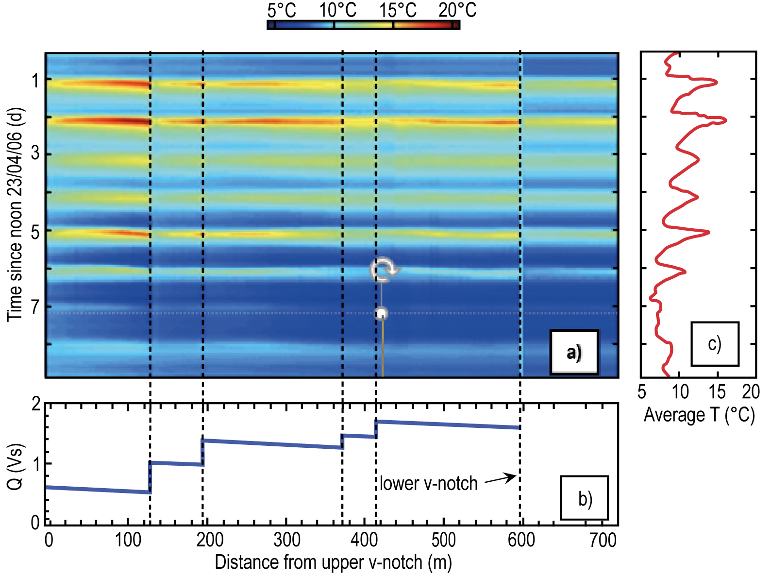
Figure 6 – a) Stream temperature in time and space from April 24 to May 3, 2006, for the first 720 m of the Maisbich in Luxembourg; b) computed stream flow with groundwater inflows at the dashed lines computed from temperature measurements, and up and downstream flow obtained from weirs; and, c) time-series of spatially averaged temperatures. The first two days (April 24 and 25) were sunny, while the last two days (April 30 and May 1) were cloudy (from Selker et al., 2006b, with permission).
Mapping the inflow of groundwater to streams was a significant advance, although this type of data could in principle be gathered from a time-consuming synoptic temperature survey using a handheld thermometer. Of more significance, however, was the use of the time-varying streambed temperature to directly calculate the volumetric flux of groundwater to the stream. Because the stream temperature had a strong 24-hour or “diel” signature, points of groundwater inflow cooled the stream during the late afternoon but warmed the water downstream during the early morning. By noting the point in time when groundwater neither warmed nor cooled downstream, the observed temperature at that point in time and space represented the true groundwater temperature, a measurement that was rarely made. Armed with this information, it was then possible to calculate, from a thermal balance model, the actual volumetric flux of groundwater entering the stream at each of these points, a measurement that could not be made with sufficient accuracy from standard stream gauging (Selker et al., 2006b; Westhoff et al., 2007). The measurement of exchange between surface waters and groundwaters continues to advance and evolve significantly with work in estuaries (Henderson et al., 2009), high-resolution vertical DTS profiling (Briggs et al., 2012), exchange in lakes (Blume et al., 2013), seepage and slope failure (Bersin et al., 2017; Schenato, 2017; Weiss, 2012; Perzimaier et al., 2007; Wu et al., 2019), and groundwater-recharge basins (Medina et al., 2020).
DTS is also now widely used to measure vadose zone processes by burying optical fiber and monitoring its temperature in response to daily/seasonal heating, or by actively heating the fiber and monitoring its thermal response (e.g., Sayde et al., 2010; Benitez-Buelga et al., 2014; He et al., 2018). In the case of daily or seasonal response, the primary variables affecting the thermal response are the rates of seepage (advective heat transport) and the soil thermal properties (primarily conductive heat transport, principally governed by the soil water content).
Work on seepage through dams and embankments relies upon the perturbation from a daily or seasonal conductive-only temperature time series. The magnitude of the advective perturbation is a function of the seepage or infiltration flux. For example, several authors (Gregory, 2009; Medina et al., 2020) calculated seepage fluxes across a large infiltration basin documenting significant spatial variability in flux rates, but also the evolution over time of the clogging of the spreading basin. Such hydraulic engineering applications of DTS continue to expand and installation of monitoring fiber is now common practice for many new dams, levees, and infiltration basins.
Developing high-resolution (both time and space) soil-moisture mapping represents a fundamental challenge in vadose zone hydrology. Most measurements are either point measurements, (measuring a volume of a few cubic centimeters), depth limited (microwave methods limited to the first 5 to 10 cm of the soil surface) or integrated sensors such as COSMOs (Cosmic-ray Soil Moisture Observing System) capable of integrating over tens of meters. By burying optical fiber, very high spatial resolution measurements can be repeatedly made. In their paper, Steele-Dunne and others (2010) first proposed to use multiple fibers, buried at varying depths, to infer soil thermal diffusivity from the phase and amplitude of daily temperature variations driven by solar heating. Soil thermal diffusivity, D, can be written as Equation 3.
| D(θ) = λ(θ)/ρCp(θ) | (3) |
where:
| θ | = | soil volumetric water content (dimensionless) |
| λ(θ) | = | soil thermal conductivity (ML1T−3Θ−1) |
| Cp(θ) | = | soil heat capacity (ML2T−2Θ−1) |
| ρ | = | water density (ML−3) |
Under the assumption that soil water content, θ, was the only soil property to be changing over time, the authors showed that soil moisture evolution could be mapped over time by estimating the soil thermal diffusivity. A publication by Dong and others (2016) improved the sensitivity of the approach by incorporating a Richard’s equation solution to improve the water content estimation resolution.
Because the soil thermal diffusivity is only weakly a function of soil water content and is also not monotonic in water content, Sayde and others (2010) adapted the soil heat-pulse sensing concept to optical fiber design. When a constant heat flux is applied to an optical fiber (typically through a distributed resistance heating element), its rate of heating is primarily a function of the soil thermal conductivity rather than the soil thermal diffusivity. Thermal conductivity is controlled by the soil-particle conductivity, soil water content and air content. The bulk soil thermal conductivity is generally linearly related to soil water content (excluding the very dry and very wet end of the soil water spectrum), and therefore any changes in time to the thermal conductivity will likely reflect changes in soil water content under the assumption that other soil properties such as dry bulk density do not significantly change over time.
Sayde and others (2010) incorporated resistance heating using the metallic armoring of an optical fiber cable and under modest rates of heating (10 W/m) noted that the cumulative heating (analogous to the total heat transfer) was strongly related to the volumetric water content (Figure 7). The relationship between water content and heating is consistent with the decrease in thermal conductivity with decreasing water content.
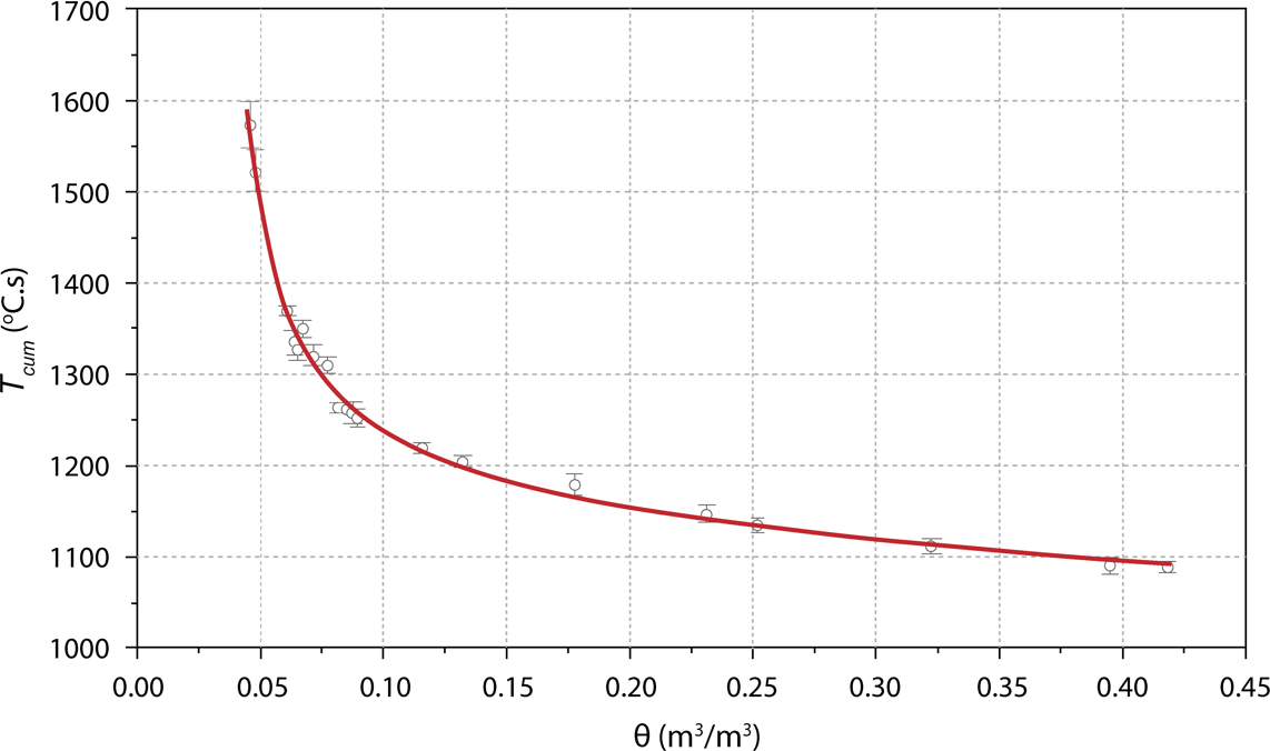
Figure 7 – The relationship between soil volumetric water content, θ and the cumulative increase in fiber temperature, Tcum for a 120-second heat pulse (with permission from Sayde et al., 2010).
Active heating of fibers in the vadose zone continues to be an evolving and very promising technique. Improvements in heating control, power requirements and analysis continue to be made (for example, as shown by Sayde et al., 2014; Ciocca et al., 2012; Sourbeer and Loheide, 2015; Dong et al., 2017; Abesser et al., 2020; and Simon et al., 2020), and as discussed next, active heating also has applications below the water table.
In a definitive article, published in 2020, on the application of active heating to cables embedded in porous media, Simon and others explored the entire parameter space surrounding the rate and duration of heat delivery, the thermal properties of the porous media, and the rate of water flow (Figure 8). It became apparent that for advection to be the dominant control of measured temperature, groundwater flux must exceed about 0.1 m/d, and to detect such a low flux rate, heating must be carried out for more than a full day. For groundwater fluxes in the 1 m/d range, heating can be as short as 4 hours, and for 5 m/d, as little as 15 minutes, using an injected energy of 20 W/m along the cable.
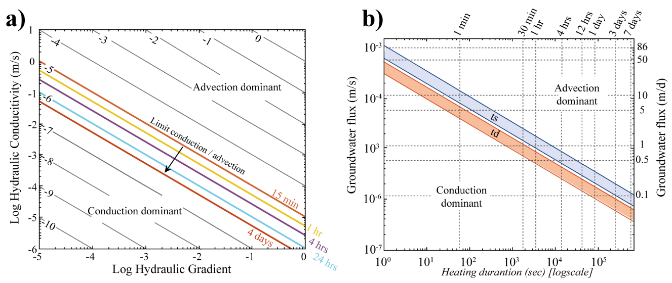
Figure 8 – a) Transition between conductive and convective heat transfer as a function of the hydraulic gradient and hydraulic conductivity (fluid velocity) and its relation to heating times of an actively heated cable. b) Heating duration versus groundwater flux.
Below the water table, DTS has been widely used to monitor thermal gradients and cross-formation flow within boreholes in thermal tracer tests (Bense et al., 2016) and monitoring ground-source geothermal systems (McDaniel et al., 2017). Bakker and others (2015) as well as des Tombe and others (2019) developed a direct-push drill system capable of simultaneously installing a loop of optical fiber for monitoring thermal tracer tests in soft sediments.
Thermal tracer tests, both short term and longer term, are optimal environments for DTS monitoring, as downhole sensor reliability is greater than traditional temperature loggers over long periods. Researchers have deployed fiber in several fractured rock boreholes and utilized both inert and thermally reactive tracers (as well as heat) to assess fracture connectivity (Hawkins et al., 2017; Banks et al., 2014). Figure 9 shows the general concept of an injection test in fractured rock, where the tracer, which could be heat, is advected through the borehole in permeable fractures.
Figure 9 – Conceptual transport of a tracer, either chemical or heat, initially injected into a borehole. The tracer is rapidly removed from the borehole in the vicinity of permeable horizontal fractures. For typical DTS applications, the tracer would be warmer water and the fractures would be delineated in the borehole DTS fiber by a localized drop in temperature over time that is more rapid than would be predicted by simple heat conduction.
Others have combined borehole heating with temperature monitoring to both estimate aquifer thermal properties in cased boreholes and horizontal fluid flux through screened intervals of the boreholes (Hausner et al., 2016). In a novel and greatly expanded use of DTS, McDaniel and others (2017) installed DTS fiber in 2,596 boreholes within and surrounding a geothermal heat exchange wellfield in Wisconsin, USA, to monitor and improve the energy efficiency of heat injection/extraction. Leaf and others (2012) conducted open-hole thermal testing; by simply injecting warm water at various depths in an open borehole. Natural flow direction in the borehole was easily measured, as was uptake into fractures. While buoyancy effects complicated the analysis, borehole flow was often downward overcoming buoyancy. Use of DTS for flow logging in wells is now well developed (Read et al., 2014; Read et al., 2015), in which a point heat source is used to inject a heat pulse into a borehole, and its dilution from inflows during heating can be mapped vertically, documenting zones of inflow to the well. Selker and Selker (2018) added the concept of heating a vertically oriented cable at discrete locations wherein the resulting heat pulses could be tracked vertically along the fiber to allow detection of both horizontal and vertical water flow.
A key challenge to borehole applications of DTS is the free advection of water within the well. Klepikova and others (2018) showed advection could be eliminated by adding 0.1 percent polyacrylamide (PAM) gel to the water in a well. This provides for a “temporary grout” of the cable so that the data reflect the aquifer characteristics rather than the movement of water within the well. Since PAM gel is soft, instruments can easily be moved through the gel as needed to take local water samples/measurements or to carry out injections of water or electrical current for tomographic studies. Following use, the PAM can be removed by slowly pumping the well.
In most of the cases described above, DTS measurements are only observing a heated or natural flow system and the actual heat transfer from the fiber is not used to infer aquifer properties. With active soil-moisture monitoring, the heat dissipation (or rise) rate from the fiber itself can be used to infer aquifer thermal properties and fluid velocities. DTS is now widely used in an active mode, in which the fiber and cable elements are heated at a known rate of heat input, and the thermal rise or decay of the temperature at the fiber and cable are used to infer aquifer or seepage properties through dams and levees (Perzlmaier et al., 2004, Bakx et al., 2019). As with active soil-moisture monitoring, a resistive heating element is incorporated in the cable system that contains one or more optical fibers. Here we depart slightly from the terminology of Bense and others, (2016) as we define active DTS in boreholes as tests that estimate aquifer properties based on heat transfer from the DTS cable to the formation or fluid, rather than heating of either the borehole fluid or rock mass and monitoring its temperature. Freifeld and others (2008) were the first to actively heat fiber in deep boreholes to estimate the vertical variation of thermal conductivity. By numerically inverting the response, the authors estimated the vertical variation of the thermal conductivity, for later use in reconstructing paleosurface temperature.
Other researchers utilized a heated-fiber system installed between the formation and a flexible borehole liner (Coleman et al., 2015; Maldaner et al., 2019). The liner reduces or eliminates vertical flow within the borehole and allows for measurement under natural hydraulic gradients. The flexible liner allows the borehole to be used for other purposes after DTS testing, similar to the use of PAM gel as discussed previously (Klepikova et al., 2018) and can be extracted after testing.
While most actively heated fibers experiments strove for uniformly heating the fiber, Selker and others (2018) constructed a spatially variable heated fiber by tightly wrapping copper heating cable at 2-meter intervals along a fiber sensing cable. This produced a higher heat flux in the tightly wrapped sections (~0.5 m) than in the remaining 1.5 m intervals where the heating cable was colinear with the sensing fiber (Figure 10). Using such a design allows for measurement of vertical fluid flow at numerous depths in a borehole and increases the practical length of cable that can be heated.
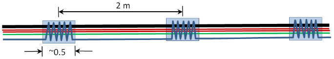
Figure 10 – Schematic of a spatially variable heated optical fiber. Wrapping of the heater cable (shown in blue) produced heating “dots” that allowed for identification of vertical flow direction and magnitude at discrete depths within the borehole.