Exercise 2
A DTS cable was installed in Martis Creek outside of Truckee California, USA, to monitor the inflow of groundwater (Avery et al., 2018). The cable ran upstream (left in the figure below) and then looped back downstream. Two well-mixed calibration baths were located at positions A and B, as shown. A long coil of cable was left in the stream at the bottom end (to the right in the figure) and a temperature sensor was placed on this coil of cable to serve as a third calibration point. Temperatures and cable positions of temperature sensors are given in the table below the figure.
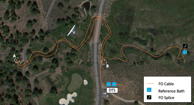
DTS cable installed in Martis Creek, California, USA.
Temperatures and cable positions of temperature sensors.
| Time | Bath “A” °C (9.68 to 25.92 m) |
Bath “B” °C (30.99 to 55.34 m) |
Downstream Cable °C (9.68 to 25.92 m) |
| 15:10:04 | 19.17 | -0.17 | 14.637 |
| 4:28:04 | 20.89 | -0.17 | 16.572 |
The cable is duplexed and was interrogated using a single-mode operation. The data for this exercise are provided in a spreadsheet that can be downloaded by visiting the web page for this book at gw-project.org/books/distributed-fiber-optic-hydrogeophysics/ and clicking the “Download” button.
- Estimate the coefficients γ, Δα and C for each DTS trace using the attached spreadsheet following the method of Hausner and others (2011) as described by Equation 2. The first trace has been calculated to provide an example and the temperature units have a conversion from Celsius to Kelvin. After the proper steps are taken to evaluate the second trace in the spreadsheet the answer will appear in cells L23-L25 in worksheet DTS RAW. It is useful to work in the the spreadsheet striving to obtain the following values and if they are not readily attained, the solution to this exercise describes the steps needed to reach these values: Time = 4:28 hours, γ = 484.28 °K, C = 1.29 dimensionless, Δα = 8.866×10⁻⁵ m−1.
- Recalculate the DTS temperatures using the calibrated coefficients and discuss how the temperatures changed.
- The calibration spreadsheet uses the spatial average Stokes and anti-Stokes values from all points on the cable within each calibration bath. It is possible to estimate the DTS temperature resolution by calculating the Root Mean Squared Error (RMSE) of the DTS calibrated temperatures within each of the calibration baths. Assuming the DTS cable was uniformly at the temperature of the calibration bath, estimate the RMSE of all cable temperatures within each bath. How does the RMSE change with distance along the cable? And why?