3 Fiber-Optic Distributed Temperature Sensing (DTS)
Heat transport in the subsurface is an important phenomenon for many hydrogeologic processes, ranging from the shallow vadose zone to the deep geologic disposal of nuclear waste. Heat transfer is usually calculated from measured temperatures or temperature fluctuations in boreholes or soils, using point sensors such as thermistors and thermocouples. These can have very high accuracies (0.001 °C) and precision (+/− 0.0001 °C).
DTS allows the inference of an optical fiber’s temperature at decimeter to meter resolution, depending on the design of the interrogator. DTS relies upon Raman scattering (where a photon is absorbed, and then a new photon is emitted, what is referred to as inelastic scattering) to infer the temperature of the material that re-emitted the photon. When a photon is absorbed and re-emitted from a Raman scattering event, the re-emitted photon will be frequency shifted either to a fixed lower frequency (termed a Stokes photon) or to a fixed higher frequency (termed an anti–Stokes photon) as shown in Figure 1. The probability of re-emitting an anti-Stokes photon increases as the scattering site temperature increases, thus the ratio of anti-Stokes to Stokes intensities in the backscatter can reveal the temperature of the location where the scattering took place. In operation, a short (multiple nanoseconds) pulse of laser light is sent down the optical fiber and, while most of the injected photons pass through the optical fiber without interacting with the fiber’s glass, some photons will undergo Raman scattering. A portion of these Raman photons will be emitted such that they are internally refracted and travel back up the optical fiber to the laser source. Upon entering the instrument, they are diverted to detectors tuned to the typical frequency shift of Raman scattering in fiber where they are counted electronically. The distance of the scattering event from the laser source is calculated from the known speed of light in the optical fiber, and the time of flight since the laser was pulsed. Photons are counted until the time of flight exceeds the known total length of the fiber. After this time, another pulse is sent down the fiber, and the process is repeated. Photons are accumulated and, analogous to seismic reflection, tens of thousands of these signals are accumulated or “stacked” to increase the signal-to-noise ratio.
The fiber length associated with each scattering event commonly termed sample spacing is a function of the pulse time of the laser and the speed at which the detectors can function (Tyler et al., 2009). For a 10-nanosecond laser pulse time, photons will travel ~2 m. If the detectors collect backscattered photons during the first 10 nanoseconds after the pulse is launched, these scattering events must have occurred in the first meter of the fiber.
DTS minimum spatial sampling or sampling interval is defined as the shortest spatial distance between successive reported Stokes and anti-Stokes measurements and is controlled by the instrument’s frequency of laser firing and the minimum sampling time for the instrument’s Stokes and anti-Stokes detectors. DTS is typically operated at the minimum sample spacing supported by the instrument manufacturer. But it is very important to understand that DTS reported temperatures of adjacent samples are not fully independent. For this reason, a spatial resolution (a performance metric for an instrument) is also specified to indicate how proximal temperature features may be distinguished and quantified. From Nyquist (1928) we know that spatial resolution is universally at least two times larger than the sample spacing, but in the case of DTS machines, these are sometimes different by as much as a factor of 10. Instrument performance as specified by its spatial resolution is typically defined as the distance between points located at 10 percent and 90 percent of the total temperature, the true temperature change at a stepwise shift in temperature along a fiber optic cable. In other words, the distance between points surrounding a sharp temperature change such that the point on the low side is not elevated by more than 10 percent of the jump and the point on the high side is elevated by at least 90 percent of the actual.
Because of dispersion of light along fiber optics, finite time for lasers to turn on and off, and limitations of optical detectors and their amplifiers to respond to changing signals, reported DTS temperatures are weighted sums of the temperatures along a cable. Laboratory tests on several systems have indicated that the weighting function is typically Gaussian, which is reasonable considering the nature of these systems. This implies that the reported value for a point x is the weighted sum of the unit Gaussian with standard deviation σ centered at x multiplied by the actual temperatures along the cable (Figure 2).

Figure 2 – Gaussian curve with a maximum of 1 and standard deviation (σ) of 1 illustrating the weighting function implicit in the 10-90 definition of DTS spatial resolution. The yellow solid line presents the reported DTS temperatures, the heavy solid black line the Gaussian weighting function over which the DTS averages in its reported temperature at position 0, and the dashed lines indicate the locations along the cable of the 10 percent and 90 percent quantiles of change in reported temperature where the true temperature change occurred at position 0 on the horizontal axis.
Selker and others (2014) explored these issues in the context of the work done by Rose and others (2013), where data were collected with a 2-m resolution DTS and sections of cable far smaller than 2 m were exposed to local heating. In general, the physics underlying DTS is very robust and worthy of study for those employing this method. For example, a DTS system must assume a certain speed of light of the original pulse and of the Stokes and anti-Stokes wavelengths. The exact speeds will depend on the exact make of optical fiber. A small deviation between actual and assumed speeds of less than 1 percent quickly leads to “dislocations” at distances of hundreds or thousands of meters along the fibers. Further discrepancy between DTS-reported position and the distance along a cable is caused by “over-stuffing” of the fiber in the cable wherein the fiber optic is longer than the cable (typically on the order of 0.3 percent or less). This is done so that if the cable experiences tension and is stretched slightly, the fiber will not experience tension. If accurate location is important, it is good practice to verify measured distances in the field by temporarily heating (or cooling) a small section of the cable. Similarly, it often pays to work directly with the measured Stokes and anti-Stokes signals instead of the temperatures calculated within the instrument using default calibration parameters. Because the DTS signals travel at different velocities and are affected differently by irregularities such as splices or acute bends (broadly referred to as differential attenuation), the raw Stokes and anti-Stokes values can be post-processed to provide a more accurate temperature.
The calculation of fiber temperature fundamentally relies upon the increasing probability of anti-Stokes interactions as the fiber temperature warms. This probability follows a Boltzmann distribution with the distribution’s exponent controlled by the scattering temperature. In practice, the Stokes and anti-Stokes photon counts are each integrated to an intensity term, Is and IaS respectively. Additionally, the overall magnitude of scattering or attenuation for both the Stokes and anti-Stokes frequencies is required to correct for the ever-decreasing number of photons available for scattering the further along the length of the optical fiber, z.
A key point here is that the greater scattering of the anti-Stokes at any location means that the rate of attenuation of light is quite different for the Stokes and anti-Stokes signals due to their different colors (wavelengths). The less-scattered red-light travels in a straight line, just as at sunset when red light is seen on the horizon while the sky directly above looks blue because the blue light from the sun is scattered towards us. Because we infer temperature from the ratio of anti-Stokes to Stokes, we must correct for the change in this ratio due to losses that occur from the location of the scattering event to the detector in the instrument. Similarly, bends and other defects in the fiber will cause different levels of attenuation of the two wavelengths. In summary, attenuation may vary along the fiber, due to manufacturing, defects, bends or connections. This difference in attenuation, usually denoted as Δα(z), for the two returning signals can be written as a cumulative integral that adds up all the differences in attenuation encountered along the optical path. The temperature (T) of the sample length can be derived (van de Giesen et al., 2012) as shown in Equation 1.
 |
(1) |
where:
| Is | = | measured photon intensity of Stokes (MT−3 or ML2T−3) |
| IaS | = | measured photon intensity of anti-Stokes (MT−3 or ML2T−3)) |
| z | = | distance along the optical fiber (L) |
| Δα | = | difference in attenuation factors between Stokes and anti-Stokes (L−1) |
| ħ | = | reduced Planck’s constant (ML2T−1) |
| Ω | = | frequency difference between Stokes and anti-Stokes scattering in typical fiber (T−1) |
| k | = | Boltzmann constant (ML2T−2Θ−1) |
| cS and caS | = | Constants related to laser power and responsiveness of the DTS detectors (MT−3 or ML2T−2) |
| λS and λaS | = | wavelengths of the Raman shifted returning light (L) as discussed by Farahani and Gogolla (1999) |
In common DTS discussions, the numerator of Equation 1 is made up of constants and is routinely shortened as γ and the first term of the denominator is replaced by a single variable, C. Equation 1 can be further simplified to Equation 2 if it is assumed that the difference in attenuation properties for the Stokes and anti-Stokes photons, Δα, is constant along the length of the fiber (Hausner et al., 2011).
 |
(2) |
As there are now several coefficients in Equation 2, it is generally necessary to have several independent temperature sensors along the length of the cable, serving as calibration points, to estimate these coefficients. These calibration points typically consist of a section of the measuring cable of a minimum length of 10 times that of the sample interval whose temperature is unchanging during each DTS measurement time. For example, ice baths or well-stirred insulated containers can be used to maintain a sufficient length of cable at a constant temperature.
It is common to construct cables to have multiple optical fibers. The first reason for this is that adding extra fibers does not add much cost to most cables. An example of a typical fiber-optic cable is shown in Figure 3. Multimode fibers allow multiple optical paths within the core and, while generally having greater attenuation, multimode fibers are commonly used for temperature sensing. Single-mode fiber allows only one “mode” of the light wave to propagate down the fiber, with fewer refraction events per unit distance and less attenuation. Single-mode fiber is typically used for distributed acoustic sensing or very long (> 20 km) DTS installations. Cables can also have a wide range of construction elements but generally, all consist of fiber(s) as well as various strength elements and plastic jacketing material.
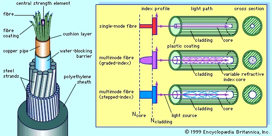
Figure 3 – Schematic of common fiber-optic cable design. Here, the fibers are encased in a metal tube (in this case copper but more commonly stainless steel). The right side of the figure conceptually shows the difference between single-mode fiber and multimode fiber, along with the differences in the nature of the interface between the two different glasses of the core and cladding glass.
“Bare” fibers cost ~US$ 0.05/m, while a fully constructed cable typically costs US$1-10/m. Installation is much more expensive per meter than the bare fiber, so it is highly recommended that at least two multi-mode and two single-mode fibers be included in any installation. This allows for more options and redundancy of the installation. One option is obtained by connecting two of these fibers at the cable’s distal end (or by looping the cable back to the instrument and connecting both ends of the fiber to the instrument), in which case the fiber is said to be in duplex mode. By interrogating in both directions and combining these signals, it is possible to calculate the spatial distribution of the differential attenuation directly and reduce the calibration parameters and calibration points to a single independent measurement (van de Giesen, 2012; des Tombe et al., 2019; des Tombe et al., 2020; Ghafoori et al., 2020).
Putting this into a larger context, it is useful to review the basic topologies for DTS cable and calibration systems, ranging from a single strand of fiber (simplex) to a looped or double fiber configuration (duplex) as shown in Figure 4. Once the geometry of the fiber is decided, the user then can decide to interrogate each fiber separately (single-ended measurement) or combine the signals from both fibers (double-ended measurement). There are pros and cons to each of these approaches. Single-ended measurements become noisier the further away from the source but require more calibration points; double-ended measurements have more noise close to the source, (Hausner et al., 2011, van de Giesen et al. 2012, des Tombe et al., 2020; Ghafoori et al., 2020).

Figure 4 – The three most common DTS fiber configurations. A single–ended measurement sends light in only one direction down the fiber, while double–ended measurements require that light be sent in both directions. Double–ended measurements require that the DTS system have at least two separate channels for fiber connection. The coiled cables in the diagram represent at least 10 measurement points on the fiber that are kept at a constant temperature.
A key consideration in designing a cable layout is the calibration and validation of the signals. First, estimating the spatial distribution of the differential attenuation, Δα, requires that calibration points are spaced along the fiber. Determination of the other two calibration parameters in Equation 2 requires two distinct zones of different temperature, all together this provides three equations to solve for these three terms.
An example set of DTS signals (or traces) are shown in Figure 5. In this example, a ~300 m singled-ended fiber had been deployed at the snow/soil interface across an area of approximately 0.5 hectares or 5000 m2 (Tyler et al., 2009). At the time of this measurement, most of the fiber was buried beneath ~1 m of snow, however, some areas had melted and the fiber ran across bare, dark volcanic soil.
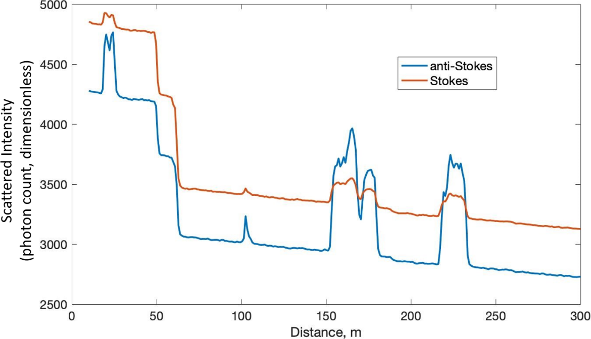
Figure 5 – Typical DTS trace from a ~300 m long fiber partially buried beneath snow. The large positive excursions in the anti-Stokes signal represent areas where the fiber was not buried under snow and exposed to direct sunlight. The sudden drops in both Stokes and anti-Stokes amplitude from 40 to 60 m are “step losses” resulting from strain on the fiber caused by sharp bending of the fiber around trees and over rocks.
Several important features common to DTS data are shown in this figure. The large positive excursions of the anti-Stokes (and to a much lesser degree, the Stokes return) represent areas where the fiber was exposed to direct sun and was warmed far above the temperature of adjacent fiber buried beneath the snow. Both the Stokes and anti-Stokes magnitude slowly decline with distance from the DTS, resulting from the loss of photons by scattering along the fiber. While this slope appears linear in Figure 5, it follows Beer’s Law of attenuation, which plots linearly on a semi-log graph. In this case, the exponential attenuation coefficient is very small resulting in a visually linear slope. Beer’s Law implies that the attenuation (or scattering of light) will follow an exponential decline with distance. Several sharp declines or downward steps in both Stokes and anti-Stokes return can be seen between 40 and 60 m from the start. These are commonly termed step losses and result from localized increases in the attenuation of light. This can be caused by simply bending the fiber such that the internal refraction is no longer sufficient to constrain the light, by microcracks or other strain, and wherever the light must pass through a mechanical connection or repair of the fiber. In Figure 5, most of the steps were caused by the fiber bending around trees and over sharp rocks, resulting in tight bends in the fiber.