Exercise 3 – Calculating Water and Solute Flux with More Dramatic Decline in Hydraulic Conductivity
Peatlands can have a variety of hydraulic conductivity distributions ranging from relatively monotonic declines with depth—as calculated in Exercise 2—to exponential hydraulic conductivity profiles. In Exercise 2, a relatively monotonic decline in hydraulic conductivity drove slight differences in the proportion of both water and contaminant transport in the upper 30 cm of peat. Under low water table conditions, the proportion of water and contaminant in the saturated upper layer (20 – 30 cm) increased while the total mass of contaminant exported to the stream decreased by ~1 order of magnitude. Peatlands with a more pronounced exponential decline in hydraulic conductivity are common and can have extremely different transport behavior.
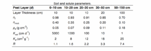
Using the same values for the following peatland hydrological parameters: Ksat (thickness weighted average = 409 cm d-1), hydraulic gradients, flow-face dimensions, peat layer depths, and water table elevations; as well as the updated hydrophysical and reaction parameters provided in the following table; calculate the proportion of water flow and contaminant under both wet and dry conditions.
Compare and contrast the peatlands in Exercise 2 and Exercise 3. Think about how the shift to an exponential hydraulic conductivity distribution affects the release of contaminants to the adjacent stream. Which change in parameters, the hydraulic conductivity or partitioning coefficient/bulk density, has a greater impact on solute transport?