Solution Exercise 1
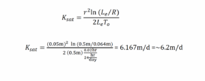
1. An Excel spreadsheet with the solution for data set # 1 is provided here. Time in seconds (column A) is expressed as hours (column B) and used to plot the data. The hourly rate is eventually multiplied by 24 to express the answer in m/d. The head measurements (h) are given in column C (m). Head recovery (H–h/H–Ho) is calculated in column D. Head recovery is plotted in log-linear space as shown in the top graph of the image below. Then a line is fit to the data. Although the data form a straight line in this case, the data often deviate from a straight line at later times; if the later points exhibit a distinctly smaller slope (see dataset #2), then follow the instructions for dataset #2. The time lag parameter (To) is interpreted from the data as the time when the line reaches (H–h/H–Ho) = 0.37. Sometimes, it is easier to work with linear-linear plots, especially when interpolating between numbers which is difficult on a log scale. The log of the head recovery values is calculated in column E. These values are plotted arithmetically as shown in the lower graph of the following image. The equation of the line can be calculated using the linear fit function of the Excel software. The value of To is estimated as x in the equation of the line by substituting 0.37 for y. The value of To is then used in the Hvorslev equation provided in exercise 1 along with the other shape parameters provided in exercise 1 to calculate Ksat, which is ~6.2 m/d. The calculation is shown in the following equation presented in Exercise 1 and the graphs are shown in the following image.
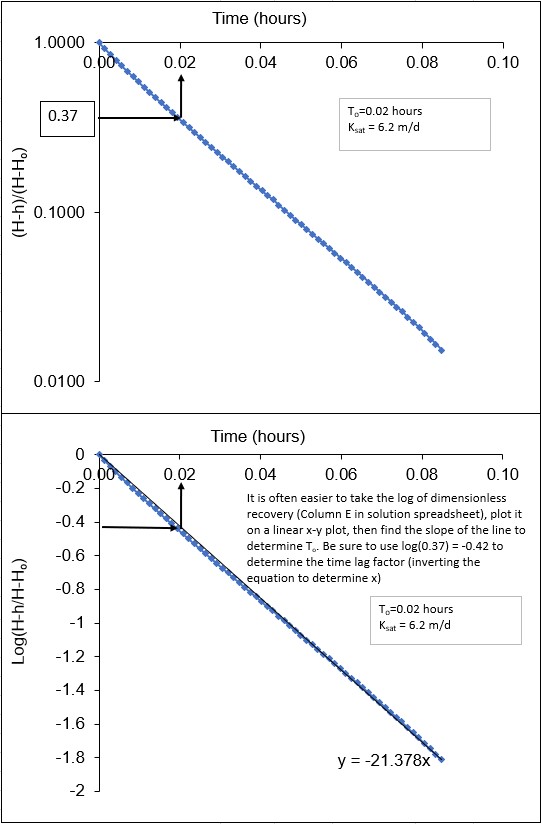
Head recovery plots for data set #1. The top graph is in log-linear space, from which To is read (To = 0.02 h). The bottom graph presents the same data plotted as log values (of head recovery) on a linear scale. To can be read from the curve or, alternatively, estimated from the equation of the line provided on the graph. Ksat is then calculated using the Hvorslev equation.
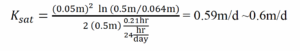
2, An Excel spreadsheet with the solution for data set # 2 is provided here. For dataset #2, the data do not plot as a straight line, likely as a consequence of peat compression caused by the large head-gradient imposed by pumping. If a straight line is fit to the entire data set, or to early-time data then the estimation of To will result in a too small time lag parameter, hence will overestimate Ksat. To obtain a more representative value, use only the late time data, thus draw a line parallel to the asymptote (i.e., latetime) head recovery curve (red line), then shift that line upwards so that it starts at the origin (1,0 in the semi-log plot) as shown in the image below (thin blue line). This rate (thin blue line) is more reflective of the actual rate of recovery after the initially rapid water inflow caused by water squeezed from collapsing peat around the intake. Read To from this line (0.21 h) and calculate hydraulic conductivity. Ksat = 0.59 m/d. To could be calculated from a slope of this new line, but it would require using coordinates estimated from the line, so it is redundant and more work than simply estimating a value of To from the line. The calculation is shown from the following equation.
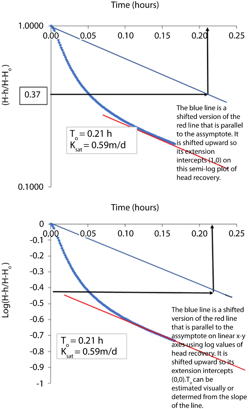
Head recovery plots for data set #2. The top graph is in log-linear space. The data do not plot as a straight line, suggesting enhanced initial recovery is not reflective of the true rate. An asymptote to the tail of the recovery curve is drawn and shifted up. The value of To is read from this line as To = 0.21 h. The bottom graph presents the same data plotted using log values of head recovery on a linear scale. To is read in the same way but using -0.43 on the y-axis which is the log of 0.37. Ksat is then calculated from Equation 5 as 0.6 m/d.