Box 5 – Mobile Water Porosity and Solute Transport
The water flux through a unit area of soil is a function of its hydraulic conductivity and the gradient across it, according to Darcy’s law. The resulting water flux has the units of velocity but is more correctly called the specific discharge, q (cm/s).
Individual molecules of water and dissolved solutes travel faster than the rate indicated by the specific discharge because the solids of the matrix do not conduct water. The velocity of water and solute molecules is faster because the volumetric rate of discharge passes only through the cross sectional area of pores. This is called the average linear porewater velocity, vL (cm/s). Therefore, vL = q/𝜙, so knowing the porosity of a matrix is key to estimating the average linear velocity of a solute passing through it. It also affects the spread (dispersion) of that solute. If there is a dual-porosity matrix—as is the case for many peat soils—estimating the average linear velocity must be done using only the mobile water porosity (𝜙mob).
Estimating 𝜙mob is not simple. One approach is to base it on the proportion of water that can be drained from a peat sample, as estimated by using water retention curves. These values vary considerably, depending on the peat’s botanical origin and its state of decomposition (e.g., Figure 16). Since the rate of solute travel is sensitive to the value of 𝜙mob, this parameter can be estimated when fitting a model of solute breakthrough data. The dispersion parameter can also be included in the fitting process. Figure Box 5-1 shows a few attempts to simulate the measured solute breakthrough data by adjusting 𝜙mob values determined from a set of water retention curves.
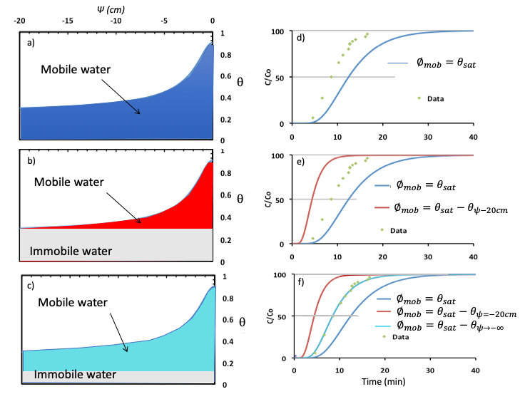
Figure Box 5-1 – A systematic illustration of the impact of using three different 𝜙mob estimates—a), b), c)— and associated water retention curves on the simulated solute breakthrough curves (solid lines) versus measured data (green points)—d), e), f)—in a laboratory column assuming no change in volume of the sample with changing pressure and drainage, and using a conservative solute. Breakthrough curves are a graph showing concentration of solute discharged from the column, expressed relative to the source concentration (C/Co), as a function of time. The breakthrough curves were simulated using the Ogata-Banks solution (Ogata and Banks, 1961). In each case, the pore-water velocity was equal to v = q/𝜙mob, where q is the quotient of discharge volume and column cross-sectional area. The breakthrough curves shown in d), e), and f) correspond to 𝜙mob illustrated in a), b), and c). In the first case (a), all water is assumed to be mobile, thus the immobile porosity 𝜙im = 0 and at full saturation (where ψ = 0) the mobile porosity 𝜙mob is 0.9. The resulting simulated breakthrough curve shown in (d) (solid blue line) is slower than the observed breakthrough (i.e., plots to the right of the measured data). In the second case (b), 𝜙im was determined by noting where the water content levels off with decreasing soil water pressure, suggesting that water can readily drain above this pressure, thus is mobile. This occurred at ψ ~ -20 cm at which 𝜙im = 0.35, thus at ψ = 0 the mobile porosity 𝜙mob = 0.9-0.35 = 0.55. Using 𝜙mob = 0.35, the simulated breakthrough curve shown in (e), solid red line) is faster than the observed breakthrough (i.e., plots to the left of the measured data). Given that these two cases bracket the observed data, it must be that 𝜙mob lies between these values. For the third simulation, 𝜙mob was estimated by adjusting it until the simulated breakthrough curve matched the observed data as shown in (f). In this case 𝜙mob is the difference between θsat and a value of 𝜙im that may reflect the water content (0.11) that occurs as ψ → –∞ (𝜙mob = θsat – θψ→–∞ ). Thus at full saturation (when ψ = 0) the mobile porosity 𝜙mob is 0.9 – 0.11 = 0.79. The resulting simulated breakthrough curve is shown in (f) by the solid turquoise line.