Exercise 1 – Determining Saturated Hydraulic Conductivity of Peat Using the Hvorslev Method
Determining hydraulic conductivity (Ksat) of peat can be done using the method of Hvorslev (1951), whose application was described by Freeze and Cherry (1979) for mineral aquifers. The method for determining Ksat in peat is identical and is based on timing the head recovery of a well or piezometer that has been bailed. The head recovery is non-linear, slowing exponentially as the water level in the well or piezometer equilibrates with the surrounding hydraulic head; thus, it should plot against time as a straight line on a semi-logarithmic plot. However, often the piezometer response in peat is not even log-linear, because a key assumption governing the response is often not valid. That is, peat is highly compressible compared to mineral sediments, so creating a large head gradient by bailing the piezometer causes the peat to compress and expel water into the piezometer rather than coming from the assumed “semi-infinite” expanse of the aquifer. This results in the pipe filling (head recovery) faster than it otherwise would, thus overestimating the “true” Ksat (Rycroft et al., 1975).
In this problem set, two data sets for bail tests in a peatland (ridge and flark of a patterned fen in northern Alberta) are provided. One has the expected log-linear response and another shows evidence of peat compression, in which there is not a log-linear response. This exercise demonstrates how to determine a reasonable Ksat value for both cases.
Bail tests involve removing water from a well or piezometer and monitoring the response. Here, we focus on using a piezometer, as the calculations are simpler because it has a fixed intake length. Comments on adapting the method to a well follow, the method being identical except for one aspect.
For a bail test, the more rapidly the water level in the pipe recovers, the higher the hydraulic conductivity. The measurements include H, which is the total hydraulic head at the start of the test (i.e., before water is removed) and Ho, which is the total hydraulic head value immediately after water is bailed from the well or piezometer (time = 0). The variable in this exercise is the time-dependent hydraulic head as the well or piezometer recovers.
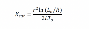
Other key values include the dimensions of the intake, including its inner radius, r, and the external radius and length of the intake: R and Le, respectively. These parameters are illustrated in the image associated with the equation for Ksat. The method of Hvorslev (1951) relies on an empirical shape factor for this type of piezometer to identify a time lag parameter, To, which is calculated as the time at which the dimensionless recovery (H–h)/(H–Ho) reaches a value of 0.37. These values are used in the following equation developed by Hvorslev to determine Ksat.

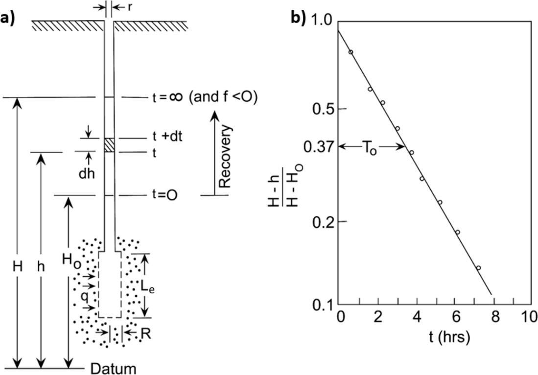
a) Identification of values H, Ho, and h, at different times (t), as well as r, R, and Le; b) Ksat is determined by the rate of recovery, which is portrayed here on a log-linear plot, from which To is estimated from a point on the line corresponding to (H-h)/(H-Ho) = 0.37. Diagram from Freeze and Cherry (1979).
As noted above, the response is commonly non-linear in particularly compressible peat. In this case, a straight line is drawn from the coordinates at the start of the test (1, 0), that is parallel to a line tangential to the asymptote of the recovery curve. This is described by Hvorslev (1951, page 41). Essentially, this approach uses the latter portion of the recovery data that better reflects the properties of the peat, rather than the initial portion that is an artifact of the test. To use this approach, plot the dimensionless recovery data (H–h)/(H–Ho) versus time, estimate the slope of the lower (ideally straighter) section of the curve, and draw a line parallel to this lower part of the curve, with its origin at 1,0 on the semi-log plot (or 0.0 on a linear plot). Then determine the time lag parameter (To) from a point on the line corresponding to (H–h)/(H–Ho) = 0.37 on the semi-log plot. Inevitably, different users will estimate a slightly different slope of the tail portion of the curve, and thus calculate different values of Ksat. The result, however, will be closer to the true value than an uncorrected estimate.
Bail tests were done on a rib and flark of a ribbed fen in northern Alberta, Canada. The piezometer intakes were both 1.81-2.31 m below local ground surface. PVC pipes with a 5 cm-inside diameter were pushed into a pilot hole to the required depth; thus, their outside diameter (6.4 cm) represents the outside radius of the tube. In these examples, a logging pressure transducer was used to record the head recovery.
- Access the data set #1 to calculate Ksat (m/d) for the piezometer located
1.81-2.31 m below ground surface in a rib of a patterned peatland. - Access the data set #2 to calculate Ksat (m/d) for the piezometer located
1.81-2.31 m below ground surface in a flark of a patterned peatland.