3.3.1 Observing Groundwater Storage Variation Over Time by In-Situ Monitoring

Groundwater levels and the volume of groundwater stored in an aquifer vary continuously over time, in response to recharge from different sources (natural recharge, artificial recharge, irrigation return flows and other anthropogenic sources), groundwater abstraction and natural discharge (regulated by system-specific characteristics). In-situ monitoring (i.e., monitoring groundwater levels in wells) forms the most direct and commonly used method to observe these variations. The water level observations are point values that in principle reveal local conditions only, but by interpolating between the data of nearby monitoring wells a spatially continuous picture of the potentiometric surface can be derived for aquifer zones that are adequately covered by monitoring wells. Sets of monitoring records that can provide an aquifer-wide picture of the groundwater storage dynamics are available for many relatively small aquifers around the world, but not for the majority of the mega aquifer systems. The enormous size of those systems makes it very difficult and costly to obtain good coverage with reasonably simultaneous field observations. Nevertheless, long-term groundwater level monitoring records with good spatial resolution and area-wide coverage are available for some of the mega-aquifer systems. This is briefly illustrated below for a few mega aquifer systems.

The first example is the North China Plain Aquifer System, 136,000 km² in extent. This is a multilayer aquifer system, with a shallow aquifer consisting of interconnected layers and separated from the deep aquifers by confining layers. The shallow and deep aquifers are hydraulically connected only in the piedmont region in the western and northern part of the plain. Gong and others (2018) derived a time series of groundwater storage anomalies for the entire North China Plain from historical monthly groundwater level data for the period 1971 to 2013. This time series indicates a prolonged declining trend of groundwater storage. On average, the volume lost from the groundwater system is equivalent to a depth of water throughout the plain of 17.8 mm/year, which corresponds to an average storage depletion of 2.4 km³/year. The anomalies are correlated with groundwater abstraction and precipitation; consequently, the average volumetric decline in equivalent depth of water throughout the plain varies between sub‑periods: 6.2 mm/year from 1971 to 1980, 20.6 mm/year from 1981 to 2002, and 18.2 mm/year from 2003 to 2015.

Yang and others (2021) created time‑series graphs for water levels in typical monitoring wells as shown for shallow and deep aquifers (Figure 15 and Figure 16, respectively) during the period from 1990 to 2020. In addition to seasonal fluctuations and variation between wet and dry years, the graphs related to the deeper aquifers show pronounced declining trends, but this is observed in only one of the selected wells in the shallow aquifer. Figure 17 shows the cumulative changes in groundwater levels over the period 1980 to 2020 for the shallow and the deeper aquifers, derived from in‑situ monitoring records (Yang et al., 2021). The groundwater levels in the deep aquifers declined more, especially in the central and eastern regions.

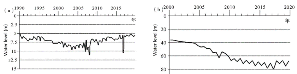
Figure 15 – Groundwater levels in typical monitoring wells in the shallow aquifer, North China Plain (after Yang et al, 2021)

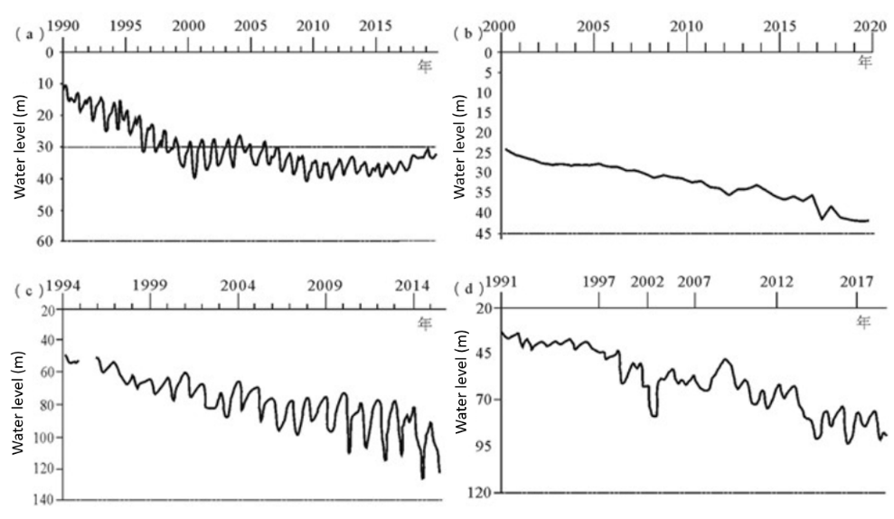
Figure 16 – Groundwater levels in typical monitoring wells in the deep aquifers, North China Plain (after Yang et al., 2021)

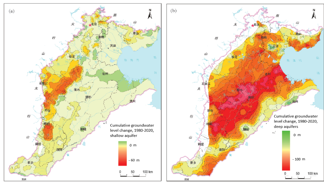
Figure 17 – Cumulative decline of groundwater levels in: a) shallow; and, b) deep aquifers of the North China Plain during the period from 1980 to 2020 (after Yang et al., 2021).

Another mega aquifer system with widespread long-term groundwater monitoring records is the High Plains Aquifer. This aquifer is 175,000 square miles in extent (around 450,000 km²) and consists of unconsolidated or partly consolidated clastic sediments of Tertiary and Quaternary age. Groundwater is generally under unconfined conditions and the saturated thickness of the aquifer varies from nearly zero to 1200 ft (366 m). Figure 18 shows cumulative changes in the groundwater levels between predevelopment time (around 1950) and 2015. This map, based on water levels from 3164 wells and other published data, shows a highly variable pattern, with zones of largest water-level declines in the southern half of the plains, where groundwater recharge is lower than in the north. Water-level changes, by well, ranged over the indicated period from a rise of 54 feet (16 m) to a decline of 234 feet (71 m), with an area-weighted average of 15.8 feet (4.8 m) decline. The monitoring data – in combination with specific yield estimates – allowed estimation of net groundwater storage depletion as 273.2 million acre-feet (337 km³) for the period from predevelopment time (around 1950) to 2015, and 10.7 million acre-feet (13.2 km³) for 2013 to 2015. In some zones, especially in Texas, the aquifer’s saturated thickness has declined by more than 50% since predevelopment (Scanlon et al., 2012; McGuire, 2017).

Figure 18 – Water-level changes in the High Plains aquifer, predevelopment (about 1950) to 2015 (McGuire, 2017).

The Indus and Ganges–Brahmaputra Basins (the mega aquifer systems 23 and 24 combined, extending over around 920,000 km²) form another large region where groundwater levels have been monitored for many years and with high spatial resolution. Most groundwater abstraction wells in this region tap from the upper 200 m of the thick series of alluvial sediments accumulated in the foredeep depression south of the Himalayas. Groundwater levels are predominantly shallow (< 5 m) and they are monitored monthly or quarterly mainly in shallow tube wells (0-100 m deep). Based on published national assessments and a subset of 2300 higher-quality monitoring records, MacDonald and others (2015) defined and mapped the long-term trends in groundwater levels (Figure 19). The map shows a significant decline in groundwater levels in the western half of the Ganges Basin and the upper part of the Indus Basin, which is strongly correlated with the areas of most intensive groundwater abstraction. On the other hand, groundwater levels in the lower part of the Indus Basin show a rising trend, driven by leakage from surface water irrigation canals (MacDonald et al., 2015). The estimated net annual groundwater depletion in the Indo-Gangetic basin amounts to some 8 km³ (MacDonald et al., 2016).

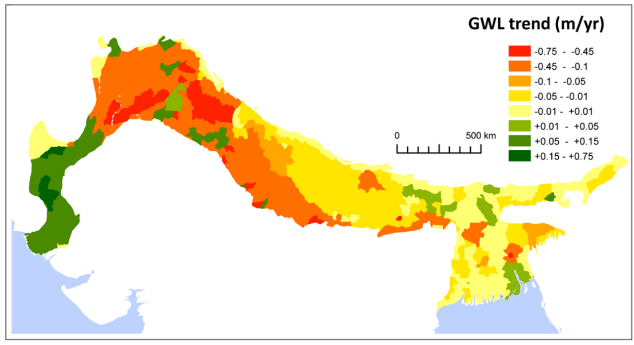
Figure 19 – Long-term trends of groundwater-level change on the Indus-Ganges-Brahmaputra basin, from high-resolution, 25-year series in situ monitoring data sets (MacDonald et al., 2015; reproduced with permission of BGS © UKRI, http://nora.nerc.ac.uk/id/eprint/511898/).

3.3.2 Groundwater Storage Variations Derived from GRACE Observations

The Gravity Recovery and Climate Experiment (GRACE) satellite mission, operational from March 2002 to October 2017, has produced a new category of data that can be used to estimate changes in groundwater storage. This innovative project monitored changes in gravity (gravity anomalies) around the globe with low spatial resolution. These anomalies can be transformed into low spatial resolution estimates of changes in total water storage (ΔTWS), from which, in turn, changes in groundwater storage (ΔGWS) can be obtained. The latter is done by subtracting estimated changes in stored surface water, soil moisture and snow/ice from the changes in total water storage. Despite many uncertainties related to the data processing and interpretation methods, these estimates provide interesting information on the variations over time of the aggregated groundwater storage in each of the mega aquifer systems. A GRACE Follow-On mission (GFO) was started in May 2018 to continue the observations. A brief overview of the history and scientific-technical principles of GRACE, as well as its application to global ground­water investigations, is presented by Chen and Rodell (2020). A recent study by Rateb and others (2020) compared GRACE estimates of storage anomalies with those from intensely monitored aquifers in the United States and found generally good agreement.

Figure 20 shows GRACE results obtained and interpreted for the High Plains Aquifer (Ogallala Aquifer, USA), as presented by Shamsudduha and Taylor (2020). The marked seasonal variation of both ΔTWS and ΔGWS is evident, while also significant interannual variation is observed, correlated with annual deviations from the long-term annual average rainfall. As could be expected, ΔGWS constitutes the lion’s share of ΔTWS, which causes both time series to be very similar. The ΔGWS time series suggests long-term groundwater storage depletion, but the time series is too short and too much dominated by seasonal and interannual fluctuations for estimating a linear trend representing the long-term depletion rate reliably and accurately. Similar time series of ΔGWS for the other 36 mega aquifer systems are presented in Figure 21 and Figure 22.

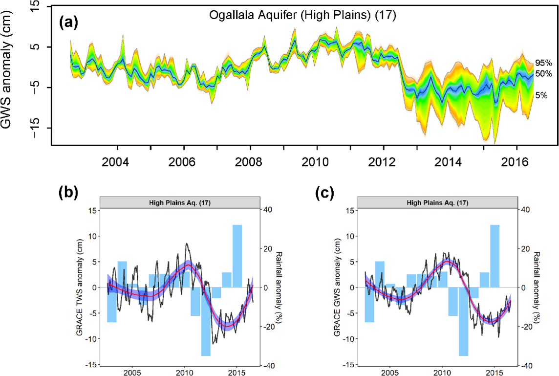
Figure 20 – Monthly time series of groundwater and total water storage anomalies derived from GRACE for the High Plains Aquifer (USA), August 2002 to July 2016: a) Groundwater storage (GWS) anomaly and range of uncertainty from 20 realizations; b) Ensemble Total water storage (TWS) fitted with a non-linear trend curve and annual precipitation anomalies; and, c) Ensemble GRACE-derived GWS fitted with a non-linear trend curve and annual precipitation anomalies (Adapted from Shamsudduha and Taylor, 2020).

Figure 21 – Monthly time series of groundwater storage anomalies derived from GRACE for the mega aquifers 1 through 19 (except number 16), August 2002 to July 2016. The ensemble GRACE-derived ΔGWS (in black) is fitted with a non-linear trend curve (the area shaded in semi-transparent gold shows the 95 percent confidence interval) and annual precipitation anomalies (i.e., percentage deviation from the mean precipitation for the period of 1901 to 2016) are shown as bars (Adapted from Shamsudduha and Taylor, 2020).

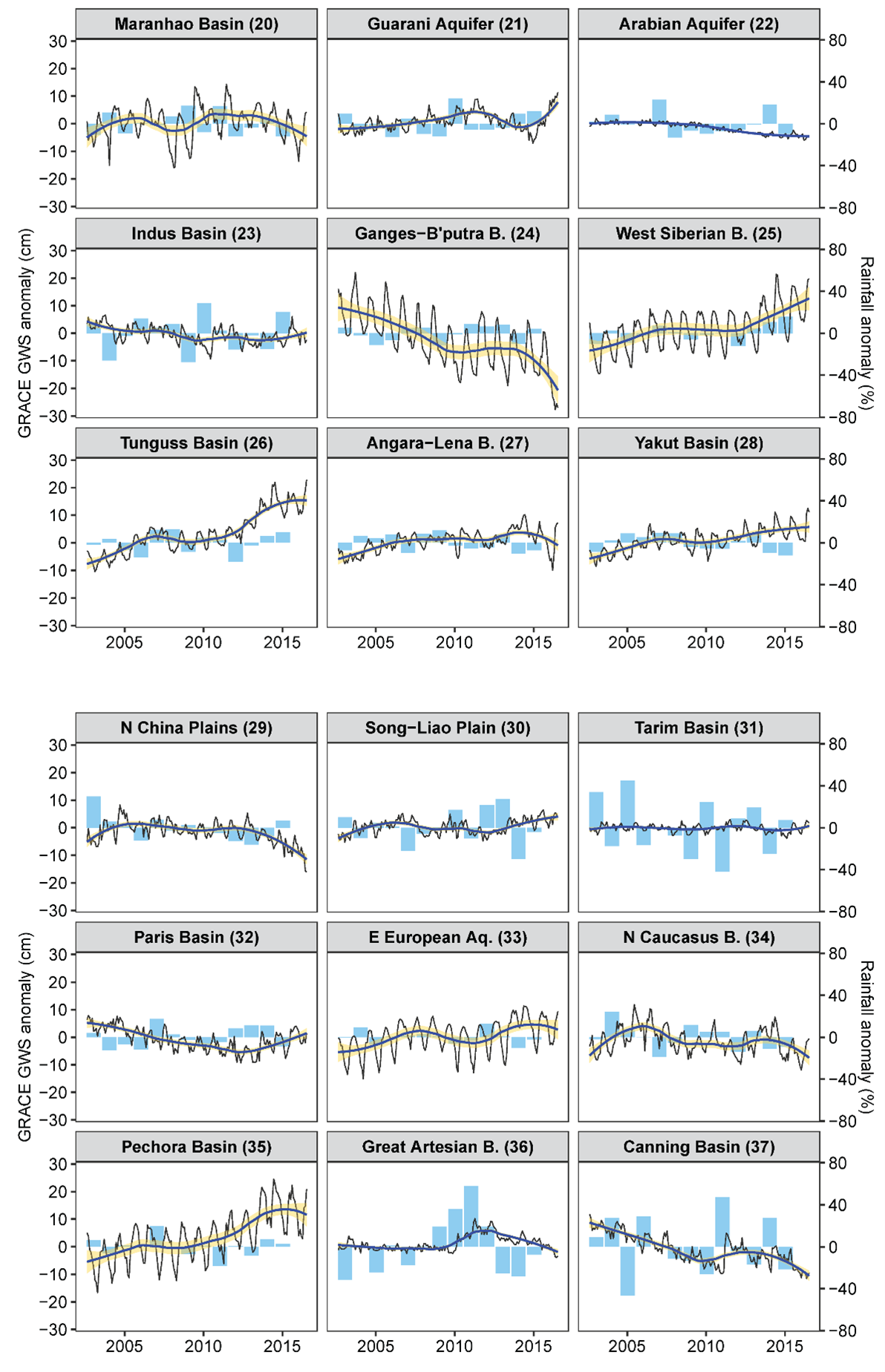
Figure 22 – Monthly time series of groundwater storage anomalies derived from GRACE for the mega aquifers 20 through 37, August 2002 to July 2016. The ensemble GRACE-derived ΔGWS (in black) is fitted with a non-linear trend curve (the area shaded in semi-transparent gold shows the 95 percent confidence interval) and annual precipitation anomalies (i.e., percentage deviation from the mean precipitation for the period of 1901 to 2016) are shown as bars (Adapted from Shamsudduha and Taylor, 2020).

The set of ΔGWS graphs for all 37 mega aquifer systems shows a diversity of groundwater storage regimes. In the first place, different intensities of seasonal variation led to large differences in the annual range of groundwater storage variation. Seasonal variation is nearly non-existent in nine aquifer systems: six in Northern and Eastern Africa (numbers 1, 2, 3, 4, 6, 9), one in Southern Africa (number 12), one on the Arabian Peninsula (number 22), and one in Central Asia (number 31). All these are located in zones with hyper-arid or arid climates. The absence of significant seasonal variation in groundwater storage in these aquifer systems is consistent with their low ranking on the recharge intensity scale (Table 7) and with their groundwater resources being classified as non- or weakly renewable. More clearly visible, but still very modest (mean range less than 100 mm) is the seasonal storage fluctuation in sixteen other mega aquifer systems: four in arid and semi-arid Africa (numbers 5, 7, 12, 13), three in North America (numbers 14, 17 and 18; in semi-arid, sub-humid and humid climates, respectively), one in South America (number 21), six in Asia (numbers 23, 26, 27, 28, 29 and 30), and two in Australia (numbers 36 and 37). The remaining twelve mega aquifer systems show a mean annual groundwater storage fluctuation range greater than 100 mm. The largest mean annual ranges are observed in the Amazon Basin (~300 mm), Ganges-Brahmaputra Basin (~220 mm), Pechora Basin (~180 mm), West-Siberian Basin (~180 mm) and California’s Central Valley (~175 mm). The seasonal variation looks regular in some aquifer systems (e.g., numbers 19, 24, 25 and 33), but irregular in others (e.g., numbers 10, 11, 15, 20 and 23).

The fitted non-linear trend curves reflect interannual meteorological oscillations: alternations of relatively dry and wet years within the period of observation. In addition, several mega aquifer systems reveal a significant overall linear trend: some of them show storage depletion (for instance, California’s Central Valley, the Ganges-Brahmaputra Basin, the North China Plain Aquifer, the High Plains Aquifer, the Arabian Aquifer System and the Canning Basin), which is in contrast with increases in groundwater storage in several other aquifer systems (in particular the Upper Kalahari, Amazon Basin, Tungus Basin, Yakut Basin and Pechora Basin). These longer-term trends can only be defined, interpreted, confirmed and explained reliably after studying in more detail the specific conditions of the aquifer systems. Analyzing information on renewable groundwater development stress (as presented in the Section ‘Interpreting and Comparing the Estimates’ and in particular Figure 14) can serve as a first step toward predicting and confirming a long-term trend.

3.3.3 Groundwater Storage Depletion

Several researchers have identified or studied groundwater storage depletion trends in one or more mega aquifer systems. Table 8 summarizes their estimates of the rate of depletion, averaged over the specified periods. The estimates are expressed both in cubic kilometers per year and in mm per year, to facilitate comparisons.

Table 8 – Estimates of groundwater storage depletion trends in selected mega aquifer systems.

References	Estimates for 21st century periods				Estimates for periods before 2000
	Period	Methods used1	Storage depletion2		Period	Methods used1	Storage depletion2
			km3/yr	mm/yr			km3/yr	mm/yr
1 Nubian Aquifer System (NAS)
Konikow, 2011	2000-2008	3,5,7	2.36	1.07	1900-2000	3,5,7	0.80	0.36
Richey et al., 2015b	2003-2013	2	6.40	2.91
Mohamed et al., 2016	2003-2013	2	0.69	0.32
Shamsudduha & Taylor, 2020	2002-2016	2	4.40	2.00
2 North-Western Sahara Aquifer System (NWSAS)
Konikow, 2011	2000-2008	5	2.20	2.16	1900-2000	5	0.53	0.52
Gonçalves et al., 2013	2003-2010	2	0.55	0.54
Richey et al., 2015b	2003-2013	2	2.86	2.81
Shamsudduha & Taylor, 2020	2002-2016	2	2.04	2.00
16 California’s Central Valley Aquifer System
Konikow, 2011	2000-2008	2,3	3.93	75.5	1900-2000	3	1.13	21.8
Scanlon et al., 2012					1860s-1961	3	1.46	28.1
Scanlon et al., 2012					1962-2003	3	1.95	37.5
Konikow, 2013	2000-2008	2,3	3.93	75.5	1900-2000	3	1.13	21.8
Faunt et al., 2015					1962-2014	9	1.85	35.6
Hanak et al., 2015					1921-2009	9	2.15	41.3
Richey et al., 2015b	2003-2013	2	0.46	8.89
Shamsudduha & Taylor, 2020	2002-2016	2	0.64	12.3
Rateb et al, 2020	2003-2017	1,2,3	1.7	33.2
17 High Plains Aquifer (Ogallala)
Konikow, 2011	2000-2008	1	11.8	26.3	1900-2000	1	2.59	5.75
Scanlon et al., 2012					1950-2007	1	5.79	12.9
Konikow, 2013	2000-2008	1	10.2	22.7	1900-2000	1	2.59	5.76
Richey et al., 2015b	2003-2013	2	-0.14	-0.31
Shamsudduha & Taylor, 2020	2002-2016	2	3.00	6.67
Rateb et al, 2020	2003-2017	1,2,3	1.2	2.67
18 Atlantic & Gulf Coastal Aquifer System
Konikow, 2011&2013	2000-2008	1,3,4,7,8	8.78	7.63	1900-2000	1,3,4,7,8	2.13	1.85
Richey et al., 2015b	2003-2013	2	6.82	5.93
Shamsudduha & Taylor, 2020	2002-2016	2	–4.93	-4.29
22 Arabian Aquifer System
Konikow, 2011	2000-2008	3,5,7	13.6	9.18	1900-2000	3,5,7	3.59	2.41
Richey et al., 2015b	2003-2013	2	13.6	9.13
Shamsudduha & Taylor, 2020	2002-2016	2	4.90	3.30
23 Indus Basin
Richey et al., 2015	2003-2013	2	1.36	4.26
Shamsudduha & Taylor, 2020	2002-2016	2	1.60	5.00
Sattar & Khalid, 2020	2005-2015	2	0.64	2.00
24 Ganges-Brahmaputra Basin
Richey et al., 2015	2003-2013	2	11.7	19. 6
Shamsudduha & Taylor, 2020	2002-2016	2	10.0	16.7
29 Greater North China Plain Aquifer System (Huang-Huai-Hai Plain)
Konikow, 2011	2000-2008	1,3,7	5.00	15.6	1900-2000	1,3,7	1.30	4.07
Richey et al., 2015b	2003-2013	2	2.40	7.50
Shamsudduha & Taylor, 2020	2002-2016	2	4.05	12.7
29a North China Plain Aquifer System (Hai Plain only)
Gong et al., 2018	2003-2015	1,2	2.53	18.6	1971-2015	1,2	2.42	17.8
Kinzelbach et al., 2021	2004-2020	2	3.32	24.4
31 Tarim Basin
Richey et al., 2015b	2003-2013	2	0.12	0.23
Shamsudduha & Taylor, 2020	2002-2016	2	0.00	0.00
Hu et al., 2019	2003-2016	2	1.52	2.93
34 North Caucasus Basin
Richey et al., 2015b	2003-2013	2	3.70	16.1
Shamsudduha & Taylor, 2020	2002-2016	2	2.61	11.3
36 Great Artesian Basin
Welsh et al., 2012					1965-1999	3	0.31	0.18
Richey et al., 2015b	2003-2013	2	–18.0	-10.6
Shamsudduha & Taylor, 2020	2002-2016	2	0.00	0.00
37 Canning Basin
Munier et al., 2012	2003-2009	2	11.00	25.6
Richey et al., 2015b	2003-2013	2	4.05	9.41
Shamsudduha & Taylor, 2020	2002-2016	2	5.16	12.0

¹ Methods adopted from Konikow (2011):
1 = water level changes times storativity, integrated over area;
2 = gravity changes over time (GRACE);
3 = calibrated flow model;
4 = confining unit analysis;
5 = pumpage data combined with water budget analysis;
6 = extrapolating fraction of pumpage derived from storage to other areas;
7 = partial record extrapolation;
8 = from land subsidence volume;
9 = unknown.

² Values as reported by authors are in roman font; values derived by conversion or interpreted from graphs are in italics. Negative values indicate an increase in storage.

The information presented in Table 8 gives rise to the following comments and conclusions.

• A diversity of methods has been used. The different methods are listed at the bottom of Table 8. As Konikow (2011) commented, methods 1 through 3 are generally the most reliable ones, but much depends on the quantity and quality of the available data, and on the skills of those who process and interpret the data. The second method (interpreting gravity anomalies observed by GRACE) has become prominent since GRACE’s introduction in 2002, but as Figure 20 through Figure 22 show, decomposition of the ΔGWS time series into its different components (long-term trend, seasonal and inter-annual fluctuations) is often not easy and rather arbitrary, and the current period of data availability (2002 to 2016) is relatively short for defining a long-term trend. GRACE and InSAR³ (that can be used in method 8) are satellite observation techniques for estimating storage depletion that complement the classical in-situ or terrestrial observation techniques on which most of the methods rely.
• Alternative depletion estimates for the same aquifer system tend to differ considerably, even if they refer to approximately the same period. The conclusion is that these estimates of storage depletion are subject to a large degree of uncertainty. Their accuracy is much lower than some researchers seem to suggest in their papers. None of the current methods of estimation produces accurate results and each has weaknesses. For example, in the GRACE method, the calculation of the ΔGWS time series from observational data is accompanied by significant uncertainty. Furthermore, as can be inferred from Figure 20 through Figure 22, it is difficult to disentangle a long-term trend from seasonal and interannual variations if the ranges of such variations are comparatively large, and/or if the total period of observation is rather small. Moving average schemes, as well as statistical and stochastic techniques for trend detection and analysis, may be helpful in this task. Analysis outcomes based on relatively short periods of observation (such as Figure 6b in Richey et al., 2015b) should therefore be presented and interpreted with utmost caution. The graph for the Paris Basin in Figure 22 is an eloquent demonstration of the importance of the length of the observation period: a trend of storage depletion would have seemed a plausible interpretation if the observation period ended in 2013, but its continuation from 2014 through 2017 makes this interpretation less credible.
• Nevertheless, long periods of observation confirm a long–term trend of groundwater depletion in several mega aquifer systems. These mega aquifer systems include the Nubian Aquifer System, the North-Western Sahara Aquifer System, Central Valley, the High Plains, the Atlantic and Gulf Coastal Aquifer System, the Arabian Aquifer System, the Ganges-Brahmaputra Basin and the North China Plain Aquifer System. Long periods of in-situ observation and hydrological data (Sections 3.2 and 3.3), contextual information and model simulations support this conclusion. Three of these aquifer systems (numbers 1, 2 and 22) are characterized by non-renewable groundwater resources, the other ones receive significant groundwater recharge, but are intensively exploited.
• A long–term linear trend (or its absence) may be hidden or be made otherwise undetectable by interannual fluctuations that last for several years. This is obvious in the case of the Atlantic and Gulf Coastal Aquifer System and the Canning Basin. In the former case, the long-term-observation record leaves no doubt about long-term depletion (which is supported by the level of renewable groundwater development stress), but climatic variability produces an apparent trend in the opposite direction during the period from 2003 to 2016 (as indicated by the GRACE record, Figure 21). The rate of groundwater depletion interpreted from the GRACE record for the Canning Basin since 2003 exceeds the rate of abstraction by at least two orders of magnitude (Table 7), thus cannot be explained by groundwater withdrawal, but most likely by climatic variability.
• Recent massive groundwater level recovery in the Great Artesian Basin may partly be explained by groundwater conservation activities. Artesian pressure (thus also the stored groundwater volume) has declined gradually in the Great Artesian Basin since the late nineteenth century, in response to groundwater withdrawal through wells. Substantial waste of groundwater was occurring for a long time by freely flowing artesian wells and a poor water conveyance infrastructure, but large government interventions beginning in the 21^st century have reduced the losses significantly, leading to partial recovery (Habermehl, 2018).

---

³InSAR is Interferometric Synthetic Aperture Radar, a geodetic technique that can identify changes in the Earth’s surface.