6.8 Plant Waters
Plants use water in their leaves, (and sometimes stems and other parts) for photosynthesis to create simple sugars and in turn all the compounds in their structure. They obtain this water, and a mixture of nutrients dissolved in the water, from the soil by absorption into their roots (Dawson et al., 2002). Describing this as use of soil water is an oversimplification. In fact, water for plant use is available from many sources, including surface water (e.g., as used by rice, mangroves, riparian plants), water in the vadose zone (e.g., water adhered to soil particles, gravitational water, and capillary water), as well as groundwater in the phreatic zone. This is further complicated by the fact that, with time, these sources may merge, separate or dry up.
Stable isotopes of H and O provide a way to discover which pools of water are being used by plants, and have the added advantage of being fairly inexpensive to analyze (especially with laser cavity instruments) and requiring small samples, therefore causing less disturbance to the soil and plants (Ehleringer and Dawson, 1992).
Caution is necessary with the use of the IRIS (isotope ratio infra-red spectroscopy) or laser instruments, as trace quantities of organic compounds in plant waters may distort the analysis and produce errors of more than 10‰ for both δ2H and δ18O. Adequate filtration to remove organic contaminants is necessary (West et al., 2010).
The basic principle of the method is to measure the isotope compositions of plant waters and potential source waters then compare the δ values to determine which pool of water the plant is using. Although this approach may work in simple situations, research over the last 40 years has shown there are many complications that may require unravelling. For example, most earlier studies assumed there was no fractionation during water uptake at the roots (Dawson and Ehleringer, 1991; Ehleringer and Dawson, 1992), although Alison and Hughes (1983) noticed fractionation and ascribed it to a 2-stage process of soil water evaporation followed by root uptake of the vapor with its evaporated isotope signature, leaving isotopically heavier water in the soil. More recent studies, have shown there is appreciable fractionation, up to 10‰ for δ2H (Ellsworth and Williams, 2007), correlated with the strength of the halophytic character of a species, or the magnitude of salt stress experienced by an individual plant (Gat et al., 2007). Non-halophytic plants may also display fractionation during water uptake, but this is dependent upon soil type and, again, the drier the soil, the more fractionation (Vargas et al., 2017). It is fairly clear that fractionation between the soil and the plant is mainly a concern in dry or salty environments, typical of deserts or in areas that experience seasonal droughts.
Large variation has also been noted in the isotope composition in different parts of the plant. This is to be expected, especially near the leaves, where transpiration causes large fractionation effects. The degree of fractionation is correlated with the transpiration rate, which is in turn influenced by higher temperature and precipitation (Pan et al., 2020) and lower relative humidity or dry conditions (Yakir et al., 1990; Bodé et al., 2019). As a result, there will be a variation in isotope composition between the water in a plant’s leaves and elsewhere in the plant, with a range of values occurring as water in the stems mixes with the fractionated leaf water. Also, over time, as transpiration varies, the degree of fractionation in the leaves will vary, and therefore any part of the plant exposed to fractionated water in the leaves will also vary. For example, Goldsmith and others (2018) found the variation in values within one tree to be similar to that between different trees.
Because of these complexities, a simple 2-point model with soil water and groundwater at each end, and one value for plant water which hopefully sits on the mixing line between the 2 source waters, is often not applicable. Instead, models have been developed to incorporate this complexity, whether it be calculation of soil water δ values (Goldsmith et al., 2018), incorporation of species-specific traits (Yakir et al., 1990), transpiration and leaf- and soil-water potentials (Cook and O’Grady, 2006) (Figure 30) or tree-water deficit, fine root distribution and soil water potentials (Nehemy et al., 2020). The choice of model then becomes a factor to consider in this kind of work (Wang et al., 2019).
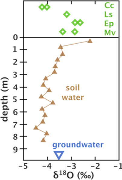
Figure 32 – Stable isotope values for groundwater, soil water and leaf water in 4 species of tree in northern Queensland, Australia. Cc = Corymbia clarksoniana, Ls = Lophostemon suavolens, Ep = Eucalyptus platyphylla, Mv = Melaleuca viridiflora. The stable isotope values were used in conjunction with transpiration rates, leaf and soil water pressure potentials to estimate the proportions of soil water and groundwater used by the 4 species (after Cook and O’Grady, 2006).
In spite of these challenges, stable isotope studies of plants have wide application in agriculture and forestry (Penna et al., 2020) and have produced some important findings, such as the proportions of groundwater versus soil water use (Dawson and Ehleringer, 1991; Cook and O’Grady, 2006), surface water versus soil water use in rice (Mahindawansha et al., 2018). They have also made it obvious that much care needs to be taken when using δ18O values in old or fossilized plant material to determine paleoclimates (Gat et al., 2007).