6 Stable Isotope Hydrology
The global water cycle is extremely complex if all the interactions with geological and biological materials are taken into account. The water cycle includes processes as diverse as weathering and volcanic eruptions in the geosphere, and organic decay and drinking by animals in the biosphere. Fortunately, the flows of water involved in those geological and biological interactions are orders of magnitude less than the major flows of water, such as evaporation from the oceans or precipitation over land, except for transpiration by plants (Jasecko et al., 2013). This global flow of water is known as the hydrological cycle. A simplified quantification of the hydrological cycle is shown in Figure 13.
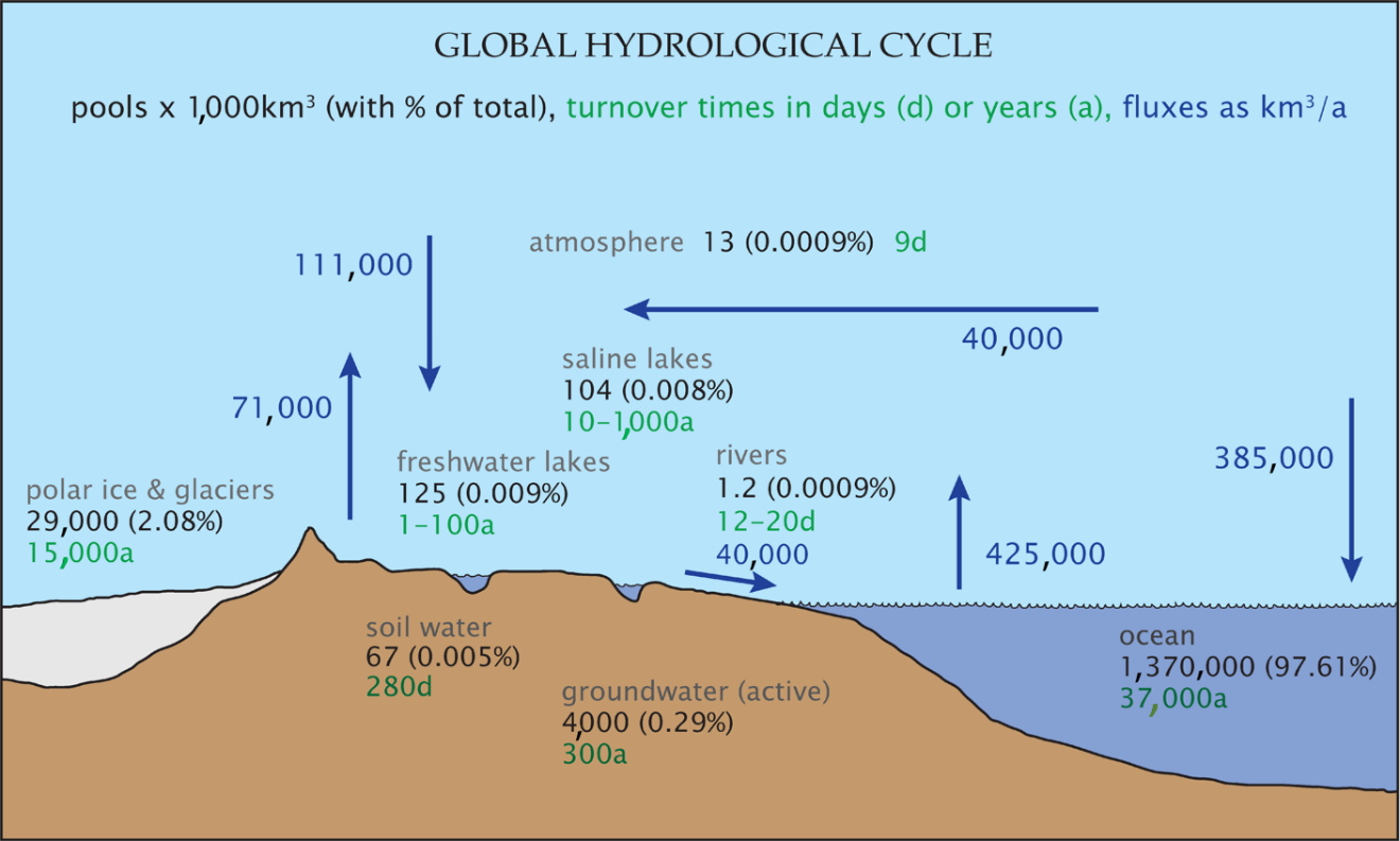
Figure 13 – A simplified quantification of the global hydrological cycle (after Reeburgh, 1994). Pools are reservoirs that store water such as the atmosphere, glaciers, lakes, rivers, soil water, groundwater and the ocean. Fluxes between pools are indicated by arrows.
Most of the fluxes from one pool to another are key points where the isotopic composition of parcels of water change. An approximation of the range of isotope compositions across the hydrological cycle is depicted in Figure 14.

Figure 14 – Estimates of typical stable isotope compositions of a variety of water sources, reservoirs and flows: δ2H in yellow, δ18O in red. Values are approximations based on information in relevant literature so, the values may differ widely from actual values for specific locations. The range of isotopic compositions shown here is less than those that occur in field settings, because these are averaged values. Nonetheless they provide an indication of the range of δ2H and δ18O values that occur in the hydrological cycle. This wide range of values, especially where there is a large change in climate, elevation or distance, is what makes stable isotopes useful for tracing water sources and movement.
With such complexity in the hydrological cycle, it is perhaps surprising that the variation in δ2H-δ18O is very defined, as shown in Figure 10 from the landmark article in Science by Harmon Craig in 1961. The most important feature of note in Figure 10 is that most precipitation has δ2H and δ18O values less than zero. This is primarily because evaporation from the oceans produces vapor that is depleted in the heavier isotopes relative to sea water (which is very similar to SMOW and has δ2H and δ18O values close to zero).
Evaporation from the oceans is a two-stage process. Initially, equilibrium fractionation occurs where water evaporates into a saturated boundary layer over the ocean surface. Then, from this saturated layer, diffusion and wind continuously remove vapor and mix it upward into the atmosphere, causing an additional kinetic fractionation (Craig and Gordon, 1965). Thus water vapor in the atmosphere is more depleted in the heavier isotopes than would occur if only equilibrium fractionation was taking place (Clark and Fritz, 1997). The measured values of δ18O in vapor over the oceans vary from about -10 to -15‰, as latitude increases (temperature decreases). These values are about 4‰ less than the equilibrium values would be. The values for δ2H are similarly lower than theoretical equilibrium values and range from -70 to -100‰ (Sharp, 2007).
Generation of atmospheric water vapor occurs mainly over the warmer oceans and it has been estimated that around 65 percent is generated between 30°S and 30°N (Peixoto and Oort, 1983). Once an air mass is cooled, either by advection over a cool surface in colder climates or by convection, the air can become saturated and condensation may commence. Condensation is dependent not only on temperature and humidity, but on the availability of condensation nuclei of the correct type (Sumner, 1988). Condensation generally proceeds slowly in response to reduced pressure or further cooling and this takes place in the presence of the vapor. In other words, cloud droplets are surrounded by vapor when they form and continuously exchange with the vapor, thus condensation is an equilibrium fractionation process.
Only general statements can be made about the causes of the distribution of isotope ratios in meteoric water because the hydrological cycle is complex. Attempts have been made to develop equations or conceptual models that can predict isotopic values for precipitation, but these have not been adequate (Sharp, 2007 and Yurtsever and Gat, 1981). However, several key factors have been identified by the first workers to interpret stable isotopes in water samples, for instance Friedman (1953), Epstein and Mayeda (1953) and Craig (1961), culminating in Dansgaard (1964). Some of these have been alluded to in previous sections. Subsequent workers continued to develop the understanding of these key factors, until they became widely accepted as a fundamental part of isotope hydrology (Gat, 1996). These factors, or isotope effects, are known as the temperature effect, latitude effect, continental effect, altitude effect and amount effect. With decreasing temperature, increasing latitude, increasing distance from the coast, increasing altitude or increasing amount of rain in a precipitation event, the isotopic composition of the precipitation becomes lighter (depleted in 2H and 18O). The cumulative result of all these effects, and others specific to local settings, can be seen in the global distribution of stable isotope compositions in groundwater, superbly collated by Jasechko (2019) and shown in Figure 15.
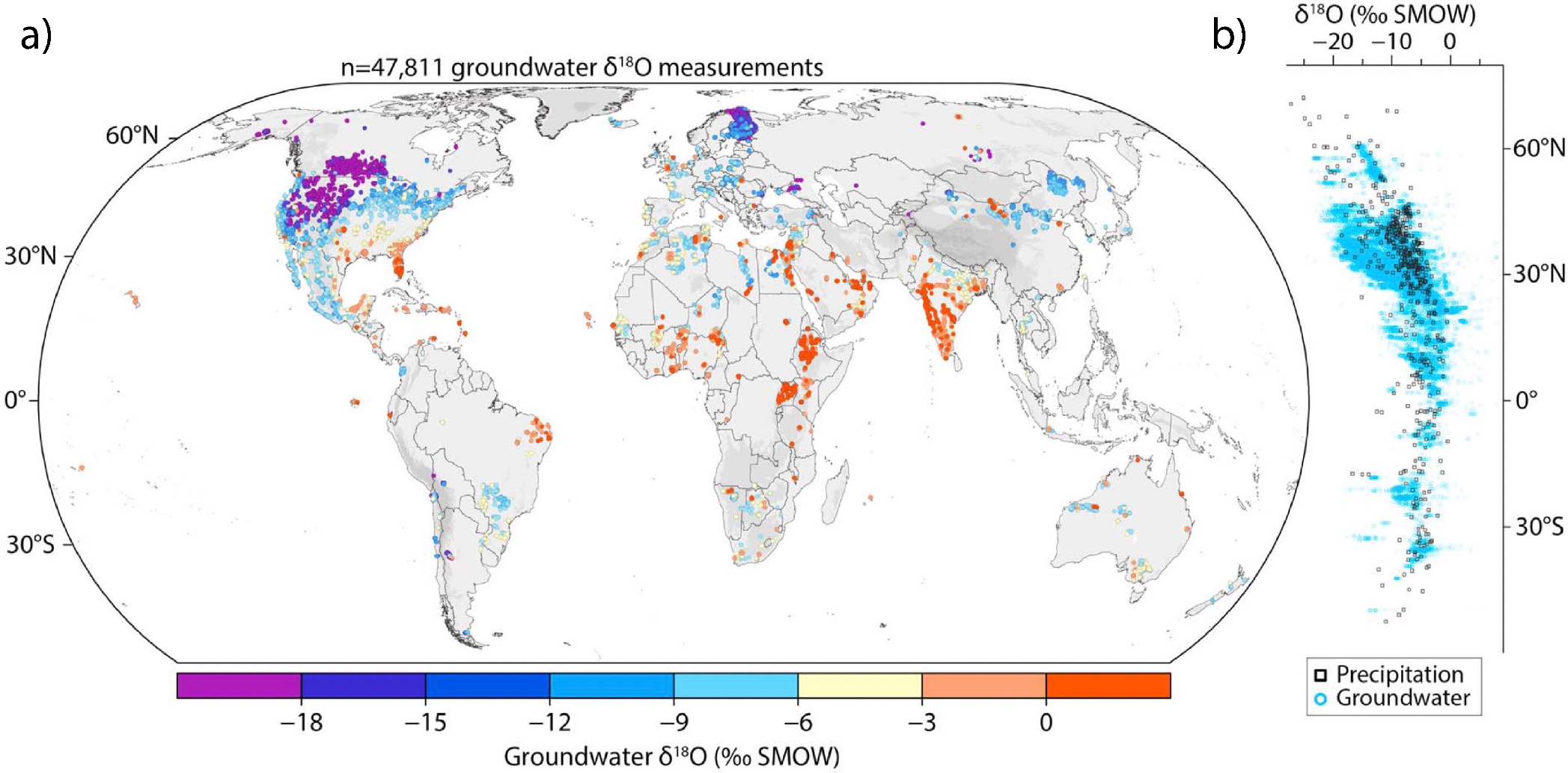
Figure 15 – Global distribution of 18O in groundwater: a) shows groundwater only; b) contains both groundwater and precipitation data. This graph summarizes nearly 48,000 measurements, from hundreds of publications over several decades. Image from Jasechko (2019).