5.8 Water Temperature
When surface water and groundwater temperatures contrast, exchange locations and, under some conditions, exchange rates can be inferred from temperature measurements (Bartolino and Niswonger, 1999; Anderson, 2005; Rosenberry and La Baugh, 2008; Webb et al., 2008; Buss et al., 2009; Boana et al., 2014). A comprehensive review of using heat as a tracer in groundwater settings is presented by Anderson (2005). Boana and others (2014) summarize the use of heat to characterize hyporheic exchange, and heat-flux/groundwater exchange modeling is described by Glose and others (2017). Examples of field applications that use VHG, seepage meters and temperature differences to characterize exchange are presented in Box 6.
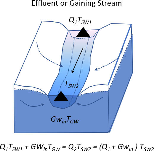
Conceptually, when seasonal or daily surface-water temperatures vary, key components of the heat budget change, one of which can be related to the exchange between groundwater and surface water as illustrated in Figure 70 (e.g., Webb et al., 2008). When parameters of the heat budget for a surface-water feature can be measured, the flux of groundwater inflow can be determined either by solving for it as an unknown in the heat budget equation or by simulating the budget and fitting the groundwater exchange term to the balance, for example as was done by Glose (2017) using HFLUX software. Schmidt and others (2007) describe the use of overall stream temperature changes to estimate groundwater discharge along a stream reach.

A basic example of using a heat budget to estimate exchange can be illustrated by examining a gaining and losing stream reach where flows and temperatures of each component are measured is shown in Figure 71. The streamflow and temperature are recorded at an upstream location and the temperature at a downstream location. These data are coupled with a measurement of the temperature of the shallow groundwater system adjacent to the stream. A mixing model is formulated with the quantity of groundwater discharging to the stream as the unknown, GWin. Other factors affecting stream temperature, such as direct surface-water heating or shading are assumed to be small and thus not included in the balance. If this is not the case, then these influences will need to be measured and included in the balance. Influent stream reaches would not be affected by the site groundwater temperature and thus over a short reach no groundwater influenced temperature changes would occur.
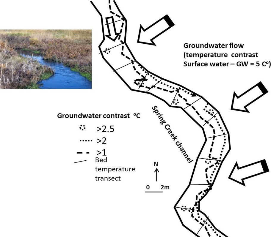
Observations of local changes in surface water, groundwater, and bottom, bank and shoreline temperatures can be used qualitatively to identify locations of diffuse and concentrated exchanges (surface water to groundwater or groundwater to surface water). Large groundwater temperature contrasts and high exchange rates make identification of exchange sites more likely. Often, daily or seasonal shifts (summer or winter) in surface-water temperatures contrast with more constant groundwater temperatures. When arrays of spatially distributed temperature monitors are installed in the bottom of surface-water features, maps of temperature contrasts can be used to infer exchange sites. For example, Loustaunau (2003) created bed-temperature transects by inserting a temperature probe 3 to 6 cm into the bed of Spring Creek near Ronan, Montana, USA (Figure 72). Groundwater was about 5°C lower in temperature than surface water. Results showed groundwater discharging along the east stream bank and areas of focused groundwater discharge were identified. Conant (2004) mapped the temperatures 0.2 m below the stream bed of the Pine River in Canada with a temperature probe in both summer and winter. He used these data to understand where a plume of contaminated groundwater was discharging to the river (Conant et al., 2019). He also used mini-piezometer measurements adjacent to temperature measurement locations to derive VHGs, performed slug tests to estimate bottom sediment hydraulic conductivities, and computed exchange fluxes (Sections 5.5 and 5.6 describe these methods).
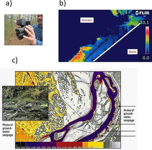
Tools to measure water temperatures include a standard laboratory grade thermometer, digital thermocouple temperature monitors with metal probes, recording stand-alone temperature monitors, thermal imaging (remote sensing) cameras, and fiber-optic distributed temperature sensing cables. When groundwater discharge temperatures and rates are sufficient to cause local changes in surface-water temperatures (e.g., cooling or warming along banks or at other locations) methods that sense changes in the surface-water temperature on a local or more regional scale can be applied. These commonly include remote sensing of surface-water temperatures using thermal imaging cameras. This can be accomplished at local site investigations by using a ground-based hand-held thermal camera, one mounted on a drone or using an aircraft mounted FLIR (Forward Looking InfraRed) imaging sensor (Figure 73). Processed images use a color scheme to present temperature contrasts and require field measurements to calibrate the temperature mapping (Cox et al., 2005). The USGS (2020) website provides a good overview of the application of thermal imaging to studying groundwater-surface water exchange. An advantage of using thermal imaging is that it provides a detailed spatial map of temperature distributions; disadvantages are that new images must be acquired to document changes over time.
When bottom temperature patterns are evaluated to assess locations of exchanges, it is advantageous to use temperature sensors embedded in fiber-optic cables that are spaced at regular distances (e.g., 1 m) for example as explained by Selker and others (2006). The cables are then sampled and measurements recorded. A good summary of how fiber-optic distributed temperature sensing (FO-DTS) methods are used to evaluate exchange is found in USGS (2016). Installation requires that the flexible cable be placed on the bottom sediment- or bedrock-water interface. It can be placed linearly (along a river channel, Figure 74) or fitted to a surface area (multiple sections (loops) of the cable covering an area being investigated). Contrasts in temperature at the bed and the surface-water temperature are computed and mapped (Figure 75). Once the cable is installed, multiple measurements can be made as long as the cable remains fixed to the bottom of the surface-water feature. Deployment of the FO-DTS method in the Columbia River at the Hanford Site, Richland, Washington, USA, identified zones of groundwater discharge near the shore during periods of low river stages (Mwakanyamale et al., 2012). However, at high river stages, indications of groundwater discharge were not observable.
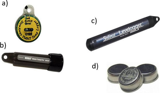
Point or single-time temperature measurements are used to identify locations and relative magnitudes of exchange. In most exchange settings, the locations and rates of exchange can vary spatially and temporally. To capture the nature of the local exchange process, individual or grouped recording sensors are required. Instrumentation can be tethered by cables to on-shore recording devices or be self-contained having internal batteries, clocks and sensors. Tethered sensors can be used in near-shore applications and where water or wave action does not damage the cable system. Most often, small diameter self-contained sensors are used to record the surface-water temperature and temperatures at multiple depths in the bottom sediments. Examples of self-contained individual sensors used in exchange studies include those shown in Figure 76. Sensors have defined temperature ranges, precision and accuracy limits; these properties must be considered when attempting to observe contrasts in groundwater and surface-water temperatures. Johnson and others (2005) provide information on the costs and operation of several sensors with a focus on their use of iButton sensors (Figure 76).
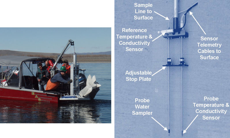
Deep water or high stream discharge may prevent placement of instruments by hand, in which case boat deployed tools can be used. One example is the Trident probe. The instrument can be pushed into the bottom sediment from a boat, and head, water quality and temperature data derived (Figure 77). It has been used to characterize conditions near freshwater and saltwater shorelines, and in large rivers and lakes. One application includes sampling of bed groundwater associated with salmon spawning areas in the Columbia River near the Hanford Site at Richland, Washington, USA.
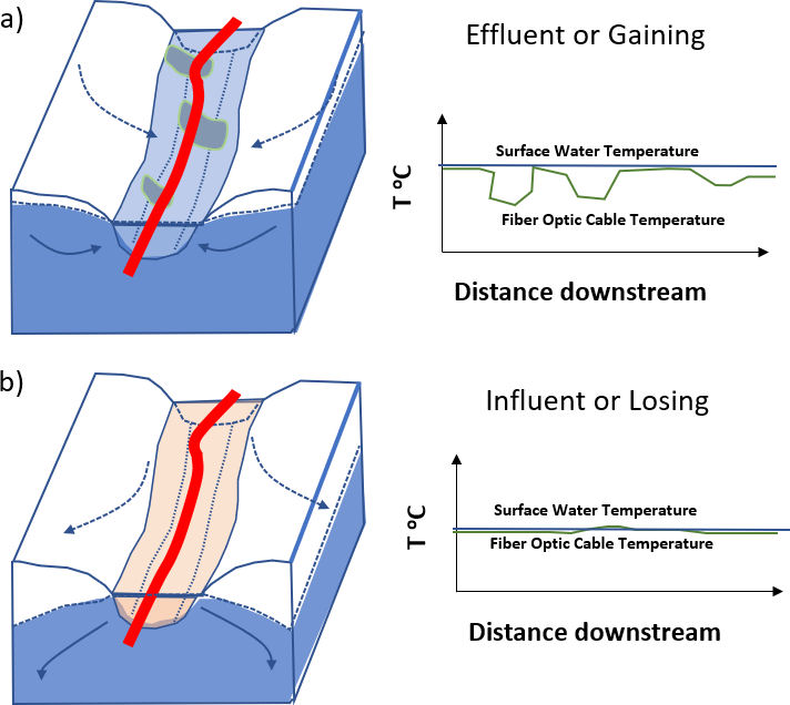
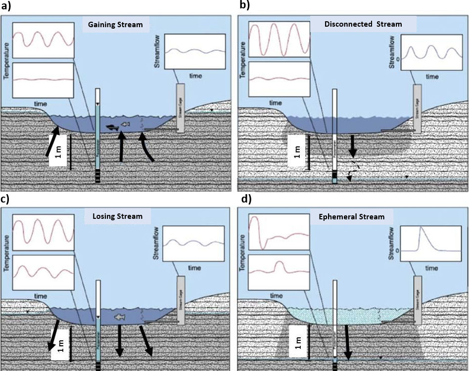
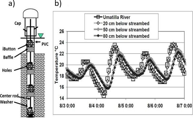
Temperature can also be used as a non-conservative qualitative or quantitative tracer of surface water or groundwater when temperature information is collected as a function of time (e.g., Stonestrom and Constantz, 2003; Anderson, 2005). This is accomplished by contrasting daily surface-water temperatures with changes in the groundwater (or hyporheic water) temperatures. Constantz (2008) described the qualitative approach to interpreting records of surface water and groundwater temperatures in the bed sediments of a surface-water body (Figure 78). A temperature monitor is placed in the surface-water feature and one or more sensors are installed in the sediments at varying distances below the bed (in the bed sediments or within a mini-piezometer) (Johnson et al., 2005; Constantz, 2008; Woessner, 2017). The paired temperature data are then analyzed to determine exchange locations and direction (e.g., Healy and Ronan, 1996; Hsieh et al., 2000; Stonestrom and Constantz, 2003; Stonestrom and Constantz, 2004; Anigoni et al., 2008; Swanson and Cardanas, 2011; Gordon et al., 2012; Constantz, 2008). Where a stream is gaining groundwater, the daily variations in the surface-water temperature (heating and cooling) are not reflected in the underlying groundwater system (Figure 78a). Instead groundwater temperatures remain relatively constant. Losing stream reaches exchange heat with the bed sediments resulting in bed temperature readings that are dampened, and off set (delayed) from the surface-water temperatures (Figure 78b and Figure 79). When surface water percolates through a vadose zone (losing stream) the groundwater temperature may not fully reflect surface-water temperature as additional heat is lost during percolation (Figure 78c). Ephemeral streams leaking water to the underlying groundwater may show a change in temperature below the bed as sediments become saturated with surface water (Figure 78d).
Field temperature data can also be used to calculate exchange rates (flux) by applying heat transport theory and modeling. Lien and Ford (2014) provide a good summary of heat flow modeling methods.
Heat is transported through porous media by flowing groundwater, dispersion and conduction (due to Brownian motion) (Stonestrom and Constantz, 2003; Anderson, 2005). During transport, heat also interacts with the solid porous media (heating and cooling). Most commonly, heat transport is modeled as isotropic, homogeneous, steady-state conditions and, in the case of groundwater-surface water exchange, modeled as one-dimensional transport (vertical) (e.g., Constantz and Thomas, 1997; Constantz, 1998; Constantz et al., 2002ab; Goto et al., 2005; Hatch et al., 2006; Keery et al., 2007; Swanson and Cardenas, 2011; Gordon et al., 2012; Bhaskar et al., 2012; Constantz, 2008; Lien and Ford, 2014; Boano et al., 2104). Modeling information is provided in Box 7.