7.  Exercises

William W. Woessner

7. Exercises

1) The conceptual models presented in this book keep conditions simple by using a constant value for hydraulic conductivity, cross sections aligned with groundwater flow lines and cross sections plotted without vertical exaggeration. Examine Figure Exercise 1 below. The cross section in Figure Exercise 1a is constructed parallel to flow, as indicated by red line (A-R-B). Under the conditions illustrated in Figure Exercise 1, think about the consequences of using head data to interpret the flow field from a cross section constructed at right angles to the stream as indicated by the line C-R-D. To make the comparison use A-R and C-R. Explain why the cross section along line A-R correctly represents horizontal and vertical groundwater flow, but head and flow data in a cross section along C-R does not appropriately represent flow conditions.

**Figure Exercise 1 –** Cross section and map view of a stream. Hydrogeologic conditions are isotropic and homogeneous and the groundwater conditions are effluent. The black ovals represent the location of monitoring wells on the cross sections. R is located where the cross sections intersect the stream. a) The cross section has no vertical exaggeration. The section is constructed along groundwater flowlines (red lines A-R and B-R) shown in (b). The left and right boundaries of the cross section coincide with the head contour of 45 (after Healy et al., 2007). b) Map view of flow field for the effluent stream. Water table contours are in blue and groundwater flowlines in black. The red line, A-R-B, shows the location of the cross section in (a). The orange line, C-R-D, is a cross section constructed at right angles to the river (Woessner, 2020).

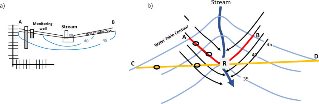
Click for solution to exercise 1

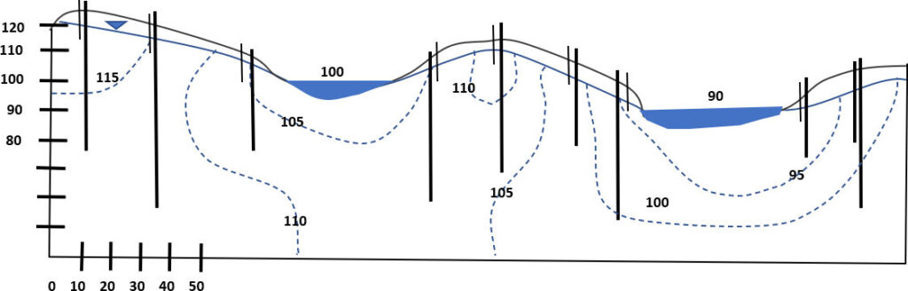
2) Examine the scaled cross section of Figure Exercise 2 showing two surface-water bodies (solid blue: rivers, lakes or wetlands) in an isotropic and homogeneous setting. Equipotential lines (dashed) were constructed from a monitoring well network containing nests of wells (vertical black lines) open only at the bottom. The water table is indicated by a solid blue line. Equipotential lines represent intervals of 5 (any units can be used).

a) Construct flowlines.

b) Label local, intermediate and regional flow systems if they are present.

c) Identify where stagnation points form and circle the locations on the cross section if they are present.

**Figure Exercise 2 –** Scaled cross section of a hydrologically isotropic and homogeneous system with two water bodies. Elevations are shown on the vertical axis and the stages of the water bodies are relative values. Black vertical lines represent monitoring well locations where head data were collected. Wells are open only at the bottom. Dashed lines are equipotential lines in 5-unit intervals (Woessner, 2020).

Click for solution to exercise 2

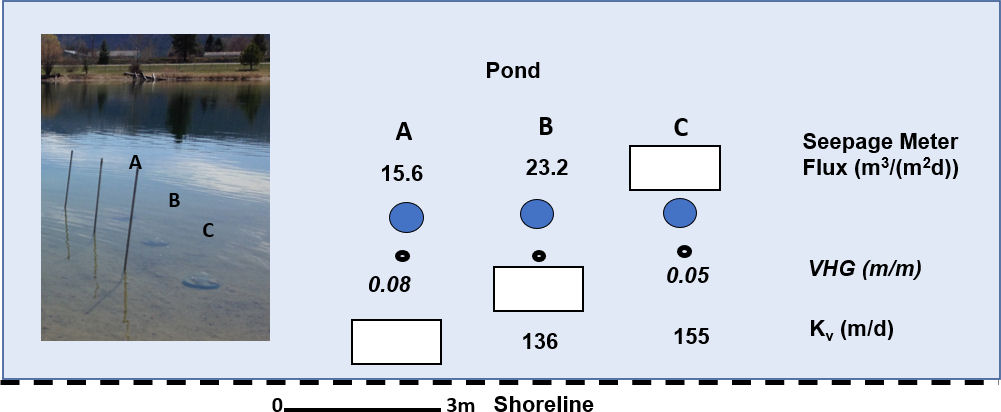
3) An exchange study of a pond was conducted by installing three seepage meters (A, B, C) and three adjacent mini-piezometers (small black open circles) as shown in Figure Exercise 3. Using the data provided compute the following:

a) The vertical hydraulic conductivity of the bed sediments at location A.

b) The VHG for B.

c) The seepage flux for C.

Figure showing an exchange study at a pond constructed in a sand and gravel aquifer — **Figure Exercise 3 –** An exchange study at a pond constructed in a sand and gravel aquifer. Three seepage meters, A, B and C (blue drums in the picture and blue circles in the map view), were installed about three meters from the shoreline. Adjacent to the meters, mini-piezometers (vertical tubes in the picture and black open circles in the map) were driven about 15 cm into the sand and gravel sediments of the bed. Seepage rates, VHG, and estimates of the bed vertical hydraulic conductivity were obtained for each of the three seepage meter locations (Woessner, 2020).

Click for solution to exercise 3

4) A water budget for a shallow subtropical lake found surface-water drainage canal discharges (34%), direct precipitation (24%) and groundwater discharge (14%) dominated inflows. Water left the lake by sheet flow into a swamp (65%), evaporation (34%), and groundwater outflow (1%). Nitrogen loading to the lake was also a concern and the lake was classified as dystropic, (chronic hypoxia and high concentrations of unionized ammonia). Groundwater was computed to deliver 48% of the load. Restoration efforts were initiated in 1996 and included removal of organic sediment, dredging and planting of native vegetation. Additional nitrogen reduction restoration is needed. The lake is in a depression created by limestone dissolution. A seepage study of the lake was conducted using twenty 208-liter seepage meters and mini-piezometers installed next to each meter (Figure Exercise 4). Meters were installed and seepage rates measured every 14 days from October through mid-May. Meters 1-14 were located in the littoral zone and 15-20 were in open water. Meters equilibrated for three months before study operation. Bags were prefilled with 1000 ml of deionized water for each seepage event. Mini-piezometers were placed in holes excavated into the bed sediment and bedrock and backfilled with sand and bentonite. Water quality samples were taken from the mini-piezometers. Mean seepage rates and total nitrogen concentrations were computed for each of the twenty sites (Table Exercise 4).

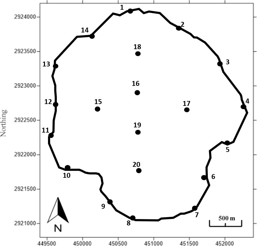
Location map of seepage meter and mini-piezometer installations in a lake — **Figure Exercise 4 –** Location map of seepage meter and mini-piezometer installations (black dots and numbers) in a lake (modified from Lucius, 2016).

Table Exercise 4 – Mean Seepage Rates and Mean Total Nitrogen Concentrations of Discharging Groundwater in a Shallow Lake. Positive seepage values represent groundwater inflow. Site numbers represent both seepage meters and the adjacent mini-piezometer (Lucius, 2016).

Site	Northing	Easting	Mean Seepage (L/m²/d)	Mean Total Nitrogen (mg/l)
1	450593.39	2924113.61	1.44	11.84
2	451291.49	2923858.38	0.26	17.7
3	451916.45	2923324.12	1.74	9.06
4	452238.73	2922714.82	1.16	4.38
5	451989.45	2922144.28	0.15	20.32
6	451695.94	2921673.69	0.2	17.1
7	451520.61	2921227.23	0.89	4.55
8	450647.05	2921081.35	7.04	5.45
9	450321.19	2921294.35	0.59	5.64
10	449740.75	2921801.64	0.14	13.02
11	449481.89	2922268.64	1.85	4.16
12	449533.30	2922725.53	-0.08	6.01
13	449535.09	2923278.14	0.25	4.74
14	450033.85	2923738.93	0.83	6.49
15	450155.54	2922664.82	0.89	52.28
16	450716.41	2922891.76	0.67	28.53
17	451418.80	2922658.34	0.87	24.27
18	450717.27	2923464.25	1.02	11.24
19	450717.90	2922308.40	3.11	23.78
20	450725.32	2921747.50	2.11	6.46

a) Plot the mean seepage data on the location map and contour it using an interval of 0.5 L/(m²d). Where is the seepage concentrated? Is water seeping from the lake to the groundwater? Would you classify the lake as effluent, influent, flow-through, or mixed? Support your answer.

b) Plot the mean total nitrogen data on a second copy of the location map. Use a contour interval of 2 mg/l. Where are the concentrations of total nitrogen the highest? Do they correspond with the highest groundwater seepage rates?

c) Compute the total mean total nitrogen loading at each location and contour the data. Use a contour interval of 20 mg/(m²d). Discuss how mean seepage meter and mini-piezometer mean water quality data can be used to target nitrogen-reduction remediation efforts. Think about what other hydrogeologic information is needed to accomplish remediation goals (Think in terms of the “big picture”).

Click for solution to exercise 4

5) Under relatively simple conditions, the temperature of stream water can be used to estimate the net gain in groundwater for an effluent reach of stream. Figure 71 presents the concept. If the streamflow at the upstream site Q1 is 2.0 m³/s and the mixed stream water temperature is 12°C, the shallow groundwater system temperature is 8.2°C, and a stream temperature measurement at the downstream site, Q2, is 10.4°C, then:
Assuming that over this 2 km river reach the other components of the heat budget are small, what is the net quantity of groundwater that discharges to this river reach?

How could individual temperature monitors installed in the stream and stream bed be used to verify the stream is gaining in this reach?

Click for solution to exercise 5

6) Heat tracing in the bed of surface-water bodies is an inexpensive and valuable tool for tracing the direction of exchanges, estimating hydraulic properties of bed material, and estimating exchange rates. USGS (2003) Circular 1260 is an excellent resource that explains the relevant principles, methods and modeling approaches. Review the document: https://pubs.usgs.gov/circ/2003/circ1260/pdf/Circ1260.pdf

a) Of the seven case studies presented, choose one and summarize the goals, methods and results. Include two key figures supporting your summary.

b) The publication also provides information on modeling of heat flow in Appendix B: “Modeling heat as a tracer to estimate streambed seepage and hydraulic conductivity” by Richard G. Niswonger and David E. Prudic. It is useful to study the appendix prior to designing field instrumentation so that field efforts will generate the required data for modeling. Read the appendix and list the parameters and boundary conditions needed when simulating heat transport from a river into the riverbed.

Click for solution to exercise 6

License