5.10 Brief Summary of Geochemical Methods
Streams, lakes, and wetlands reflect the chemical composition of the sources of water exchanging with the landscapes and hydrologic systems connecting them. For example, the chemical composition of an effluent lake will reflect the precipitation/runoff and evaporative concentration chemistry as well as chemical inputs from stream and groundwater discharges. A discharge wetland may be dominated by the chemistry and evapotranspiration of groundwater input. The geochemical principles used to identify groundwater-surface water exchange such as characterizing source waters, tracing changes in groundwater quality along flow paths, and interpreting flux and velocities, are described in a wide range of hydrogeology, hydrology and geochemical texts (e.g., Freeze and Cherry, 1979; Fetter, 2001; Fritts, 2012; Drever ,1997; Stumm, 1996; Brezonik and Arnold, 2011; Cook and Herczeg, 2000). These texts and other resources also address proper geochemical sampling and analytical methods. Detailed discussion of these concepts and methods are beyond the scope of this book.
Common geochemical techniques applied to deciphering groundwater-surface water exchange include mass balance geochemical mixing modeling, application of stable and radioactive isotope data to differentiate water histories and sources, and use of natural and introduced environmental tracers.
When groundwater and surface water chemistries contrast, components of groundwater-surface water exchange may be detected by evaluating waters for variations in concentrations of ionic constituents, stable and unstable isotopes, organic compounds, dissolved oxygen, pH, temperature, and total dissolved solids (TDS) or specific conductance. Healy and others (2007) list examples of constituents that are useful in water-budget/mass-balance models that often occur in contrasting concentrations in surface water and groundwater (Table 2).
Table 2 – Examples of Tracers Used in Chemical Water Budget Studies (after Healy et al., 2007).
| Use | Natural occurring in environment |
Historical added to environment during past human activity |
Applied introduced for testing |
Example Study |
| Groundwater age time since recharge water isolated from atmosphere |
35S, 14C, 3H/3He, 39Ar, 36Cl, 32Si
|
3H, 36Cl, 85K, chlorofluorocarbons, herbicides, caffeine, pharmaceuticals | Plummer and others (2001) | |
| Recharge Temperature | N2/Ar solubility | Plummer (1993) | ||
| Tracing groundwater flow paths |
18O, 2H, 13C, 87Sr
|
Chlorofluorocarbons, herbicides, caffeine, pharmaceuticals | Cl, Br, dyes | Renken and others (2005) |
| Exchange groundwater surface water |
18O, 2H, 3H, 14C, 222Rn
|
Cl, Br, dyes | Katz and others (1997) | |
| Distance and Travel Time of surface water |
Cl, Br, dyes | Kimball and others (2004) |
A mass balance or chemical mixing model of exchange between a surface-water system and the associated groundwater system can be used to identify exchange components (Figure 82). For example, a mixing model for a lake under steady-state conditions that is solved for the rate of groundwater inflow would be formulated as shown in Equation 7.
 = =  |
(7) |
where:
| GWin | = | groundwater discharge to the lake (L3/T) |
| GWout | = | flow of lake water into the adjacent groundwater (L3/T) |
| SWin | = | flow of surface water into the lake (L3/T) |
| SWout | = | flow of surface water out of the lake (L3/T) |
| PPTin | = | precipitation falling onto the lake (L3/T) |
| Eout | = | direct evaporation from the lake (L3/T) |
| CXXxxx | = | Concentrations of a selected constituent in component XXxxx, such as CSWout (M/L3) |
Mixing models can be formulated using a single species or component, or ratios of constituents. Healy and others (2007) and Winter (1981) caution that if some components of mass balances are poorly defined, large errors are likely. An example of a mixing model application is presented in Box 9.

In some settings, changes in water chemistry along a groundwater flow path can be used to estimate flow rates. For example, in situations where surface water freely infiltrates the hyporheic or groundwater system the concentration of radon (222Rn) buildup along the flow path is used to establish infiltration rates and sources of water. Most surface-water features have low concentrations of radon as they are open to the atmosphere. Once this water infiltrates, natural radon produced in the sediments is incorporated in the water and concentrations increase until equilibrium is established (e.g., Baskaran et al., 2009; Sacks et al., 1998). Hoehm and Cirpka (2006) describe the use of radon to assess residence times of surface-water exchange in floodplains of the Southern Alps.
Another useful approach is to apply mixing models to constituent concentrations along shorelines and within stream systems to examine sources and contributions of water. Smerdon and others (2012) discuss the use of multiple isotopes to identify water sources and quantify base flow along a 60 km section of the tropical Daly River, Australia. Isotopes of radon (222Rn), sulfur (SF6), helium (4He), as well as chlorofluorocarbons (CFCs) were sampled to characterize spring discharges along the channel, the main channel chemistry, and the adjacent groundwater chemistry. Regional groundwater contained concentrations of 4He and very low concentrations of SF6 and CFCs suggesting long residence times on the order of 10,000 years. Base flow generated by local springs was dominated by SF6 and CFCs suggesting more localized groundwater exchange. Based on the concentration of constituents in the base flow, they concluded that over 45% of the base flow originated from regional groundwater flow.
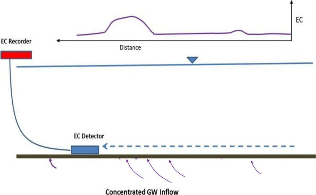
Field methods have also been developed to identify exchange locations using geochemistry of pore water in bed sediments (Lee, 1985; Vanek and Lee, 1991; Lee et al., 1993; Harvey et al., 1997; Cey et al.,1998; Kennedy, 2017). The approach uses a conductivity probe to map changes in electrical conductivity (EC) along the bottom sediments of a surface-water feature (Figure 83). This method is used to obtain multiple bed conductivity transects and map contrasts between electrical conductivity of pore water in bed sediments and adjacent groundwater (e.g., Harvey et al., 1997).
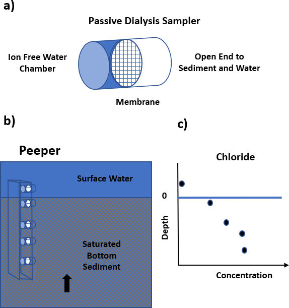
When exchange rates in fine-grained bed sediments are low, passive diffusive-membrane geochemical samplers can be used to collect pore water sediment samples. These samplers allow pore water to diffuse into one or more collection chambers (Figure 84).
Pore-water profiles are often used to examine geochemical processes at the sediment-water interface. However, they can also be used to examine the slow transport of conservative constituents between surface water and groundwater. These data sets are examined to determine locations and exchange rates using transport models (e.g., Freeze and Cherry, 1979; Zheng and Bennett, 2002). An example of a geochemical model used to explore transport though a lakebed is provided by Cornett and others (1989).
Several types of passive samples have been developed for sampling both general ionic chemistry and to target specific inorganic and organic contaminants (e.g., Burgess et al., 2016). The United States Environmental Protection Agency has published an informative manual on the use of passive sediment pore water samplers (Burgess et al., 2016). Samples use low-density polyethylene (LDPE), polyozymethylene (POM), polydimethylsilozane samplers (PDMS) for hydrophobic organic chemicals, and diffusive gradient thin films (DGT) for selective metal evaluations. They provide a table of material used in samplers and suppliers. Care in selecting both the composition and methods of installation are required to obtain representative data.
The chemical composition of pore waters can also be sampled by extracting groundwater from mini-piezometers and pore water from sediment cores. A method to extract and analyze pore water from sediment cores collected in Lake Baldegg, Swizerland, used MicroRhizon samplers and capillary electrophoresis methods (Torres et al., 2013).