Solution to Exercise 6
6) Heat tracing in the bed of surface-water bodies is an inexpensive and valuable tool for tracing the direction of exchanges, estimating hydraulic properties of bed material, and estimating exchange rates. USGS (2003) Circular 1260 is an excellent resource that explains the relevant principles, methods and modeling approaches. Review the document: https://pubs.usgs.gov/circ/2003/circ1260/pdf/Circ1260.pdf
SOLUTION:
a) Of the seven case studies presented, choose one and summarize the goals, methods and results. Include two key figures supporting your summary.
The table of contents of the report is presented here.
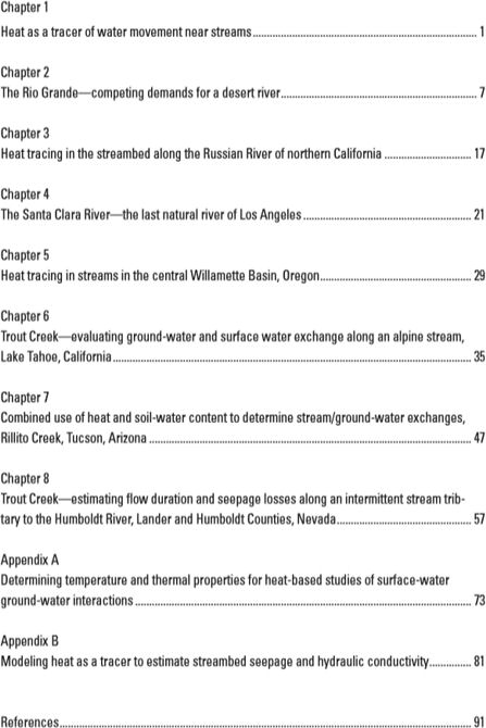
As an example, here is a summary of the report presented in Chapter 6. Trout Creek (Allander, K.K., 2003).
Purpose: To develop information on the magnitude and timing of groundwater discharge and the corresponding groundwater nutrient load to tributaries of Lake Tahoe. Trout Creek was chosen for groundwater exchange evaluation because creek flows provide the second largest stream nutrient sediment load to the lake. It is urbanized in the lower reach, has on-going monitoring, and has undergone channel restoration in the urban reach.
Methods: Along selected study reaches: Streamflow discharge measurements (synoptic surveys); monitoring well water level measurements in shallow monitoring wells installed in the channel and fitted with transducers; streambed temperature measurements using thermocouple sensors at two sites at 5 depths below the stream bottom (to 2.1 m).
Results: Water level differences between the monitoring well and stream stage varied seasonally (see Figure 7 copied below).
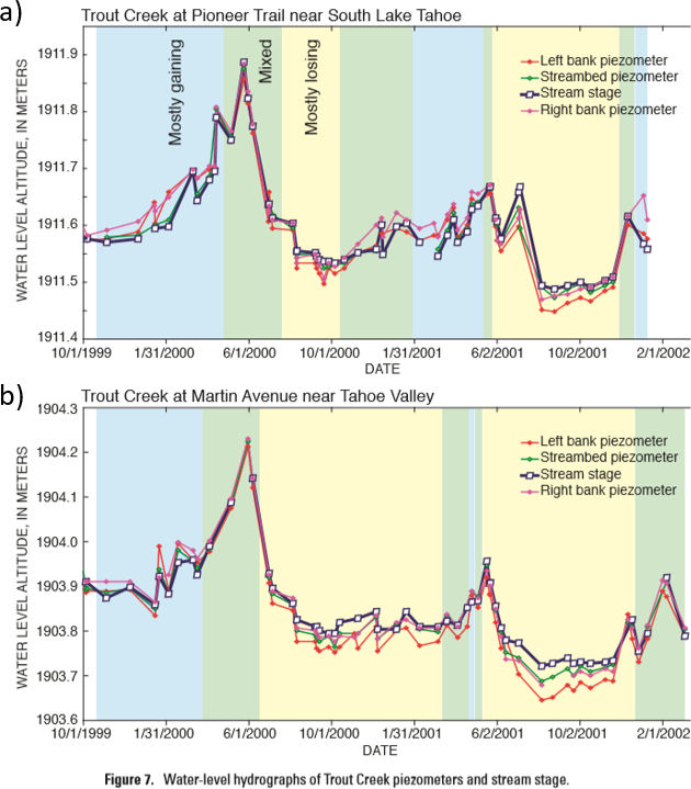
The exchange process varied seasonally as indicated by VHGs measured in piezometers.
Summary: Study results showed a dynamic exchange process. Groundwater generally contributes to streamflow in the winter and early spring (blue on Figure 7), and the stream mostly loses flow to the groundwater in the summer and fall (yellow on Figure 7). The next step is to combine groundwater exchange with nutrient concentrations to produce loading information.
b) The publication also provides information on modeling of heat flow in Appendix B: “Modeling heat as a tracer to estimate streambed seepage and hydraulic conductivity” by Richard G. Niswonger and David E. Prudic. It is useful to study the appendix prior to designing field instrumentation so that field efforts will generate the required data for modeling. Read the appendix and list the parameters and boundary conditions needed when simulating heat transport from a river into the riverbed.
Example of Model Set up, boundary conditions and features:
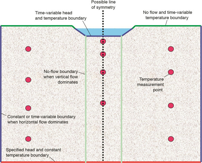
Surface Boundary
Specified head and time variable temperature
Bottom Boundary
Specified head and constant temperature
Initial Conditions
Initial estimates of heads and temperatures at the beginning of the modeling
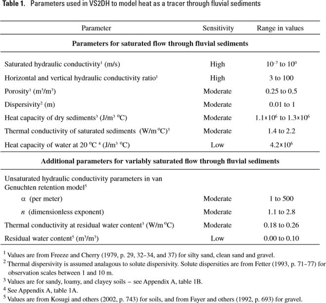
Model parameters
Example of parameters in Table 1 (Appendix B).
Observation Data
Spatial and temporal distributions of head and temperatures to be used as initial conditions and in model calibration.