5.5  Surface-water Stage and Groundwater Monitoring Networks

William W. Woessner

5.5 Surface-water Stage and Groundwater Monitoring Networks

Installing a monitoring-well and surface-water-stage network allows for collection of head and stage data to generate two- and three-dimensional equipotential distributions. Interpretations of these data yield groundwater flow directions, rates, and changes in heads over time. Two-dimensional maps and cross sections, three-dimensional renderings, as well as model simulations and associated graphics provide visualizations of exchange conditions.

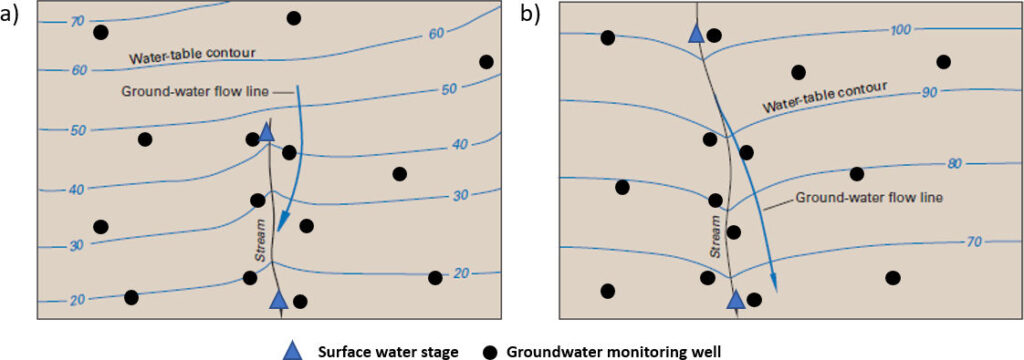
Map views and cross sections showing head and stage distributions allow groundwater flow directions and exchange conditions to be inferred (Figure 58). Groundwater elevations are derived from wells penetrating the associated, usually shallow, unconfined groundwater system. Networks of monitoring wells or piezometers are established using either existing wells or specifically-installed, small-diameter (~5 to 10 cm) wells. Well designs usually include a short, slotted section near the bottom of the well, a cap on the bottom of the well, and closed piping extending to the surface (Figure 59) (e.g., Sterrett, 2008). Other well designs are appropriate when installation conditions are difficult or budgets are restrictive (e.g., hand driven sand points, jackhammer-driven tubes, and jetted piezometers; Sterrett, 2008).

**Figure 58 –** Schematic of monitoring well networks and stream stage stations used to assess groundwater-stream interaction. Geologic information, head data, and river stage elevations are used to construct an equipotential map (blue lines and relative numbers) and generate groundwater flow lines (assuming steady state, isotropic and homogeneous conditions). a) Gaining stream. b) Losing stream connected to the water table (modified from Healy et al., 2007).

Figure showing a typical groundwater monitoring well design — **Figure 59 –** Typical groundwater monitoring well design. The cement surface seal and low permeability annular seal material limit the leakage of surface-water runoff around the well casing. The filter pack is typically a higher hydraulic conductivity material that facilitates the movement of water to the portion of the well open to the groundwater system (the well screen in this example) (Woessner, 2020).

In most cases, wells are installed in the unconfined groundwater system interacting with the surface-water feature. In addition to wells completed near the water table, a portion of the wells should be paired with one or more deeper wells to measure the direction and magnitude of vertical hydraulic gradients (Figure 60). Gradients are computed as the difference in heads (100-105 in Figure 60) divided by the difference in well depths (30 in Figure 60). The gradient’s negative sign shown in Figure 60 is a convention indicating that flow is from areas of high to low hydraulic head. Thus, when Darcy’s Law is used to generate groundwater discharge, flux, velocity or estimates of hydraulic conductivity, gradients are computed by subtracting the head at some distance down gradient from the head at the starting point. Woessner and Poeter (2020) discuss the use of Darcy’s Law to quantify flow and provide further detail on the convention for calculating gradient in Section 4.3 of the Groundwater Project book titled “Hydrogeologic Properties of Earth Materials and Principles of Groundwater Flow”. The vertical movement of groundwater is described as upward (head in deep piezometer is greater than head in shallow piezometer) or downward (head in deep piezometer is less than head in shallow piezometer). Multiple monitoring well depths at a location also allow for detailed water quality sampling and aquifer property determination.

Figure showing pairs of shallow and deep monitoring wells — **Figure 60 –** Pairs of shallow and deep monitoring wells provide information on vertical gradients for an effluent condition. Equipotential lines are dashed, and groundwater flow arrows are shown in dark blue. Flow direction interpretation assumes isotropic and homogeneous conditions. There is no vertical exaggeration in this section. Water levels in open-ended monitoring wells are shown in light blue. The vertical gradient at location A would be computed as the difference in heads between wells 2 and 1 (orange arrows) (in this case 100-105=-5) divided by the distance separating the ends of the piezometers (L₂-L₁, green arrows), DL=30, -5/30=-0.17(Woessner, 2020).

Water levels in monitoring wells are determined using steel or electric water-level measuring tapes, transducers, and/or acoustical tools. The tops of the well casings, from which water levels are measured, and adjacent stream stage stations are surveyed to a common datum for the study area (e.g., mean average sea level). The elevation of groundwater levels, streams, lakes and wetlands are typically determined by standard surveying techniques (e.g., level, theodolite, survey grade GPS). Survey errors should be sufficiently small so that differences between stages and groundwater elevations are identifiable at the relevant scale of investigation.

Water level data are contoured, and groundwater flow lines mapped using methods appropriate for the identified anisotropy in aquifer materials (e.g. Woessner and Poeter, 2020). Representations of groundwater flow in cross sections need to account for both cross-sectional vertical exaggeration and anisotropy (e.g., Freeze and Cherry, 1979; Anderson et al., 2015; Woessner and Poeter, 2020). Monitoring well designs should also accommodate likely water quality sampling tools and methods, and be made of materials that do not compromise groundwater geochemistry (e.g., Sterrett, 2008). The extent of the well network is based on the domain boundaries and the importance of the far-field groundwater conditions (requiring wells farther from the site-specific study site) to describe exchange (e.g., Anderson et al., 2015).

To determine vertical gradients between a surface-water body and the groundwater using an inexpensive tool, small diameter tubes (often less than 2.54 cm diameter and a meter or two long) can be installed to various depths directly in the bed of the surface-water feature. They can be installed as a temporary instrument or left in place for future measurements. Most commonly, these mini-piezometers are placed below the unconsolidated bed of the surface-water feature to examine the distribution of vertical gradients (e.g., Lee and Cherry, 1978; Simonds and Sinclair, 2002; Cox et al., 2005; Buss et al., 2009). The Rosenberry and others (2008) publication is an excellent reference describing mini-piezometer design and use.

License