Box 2 – Review of Darcy’s Law
Darcy’s Law (Equation Box 2-1) states that the volumetric flow rate (discharge) of groundwater in a porous material is 1) directly proportional to the difference in hydraulic head between two locations, 2) indirectly proportional to the length of the flow path between those locations, and 3) directly proportional to the area through which flow occurs. The proportionality is converted to an exact equation by including a proportionality constant, in this case, the hydraulic conductivity. Darcy’s Law is illustrated in Figure Box 2-1. Darcy’s Law dictates that heads will decline linearly in a homogeneous material with a uniform flow area as shown in Figure Box 2-2.
Q = hydraulic conductivity ×  × area = KiA × area = KiA |
(Box 2-1) |
where:
| Q | = | volumetric flow rate (L3/T) |
| K | = | hydraulic conductivity of the porous medium (L/T) |
| i | = | hydraulic gradient in the direction of flow, which is h2 – h1 of Figure Box 2-1 divided by the distance between the heads (dimensionless L/L) |
| A | = | area perpendicular to the direction of flow (L2) |
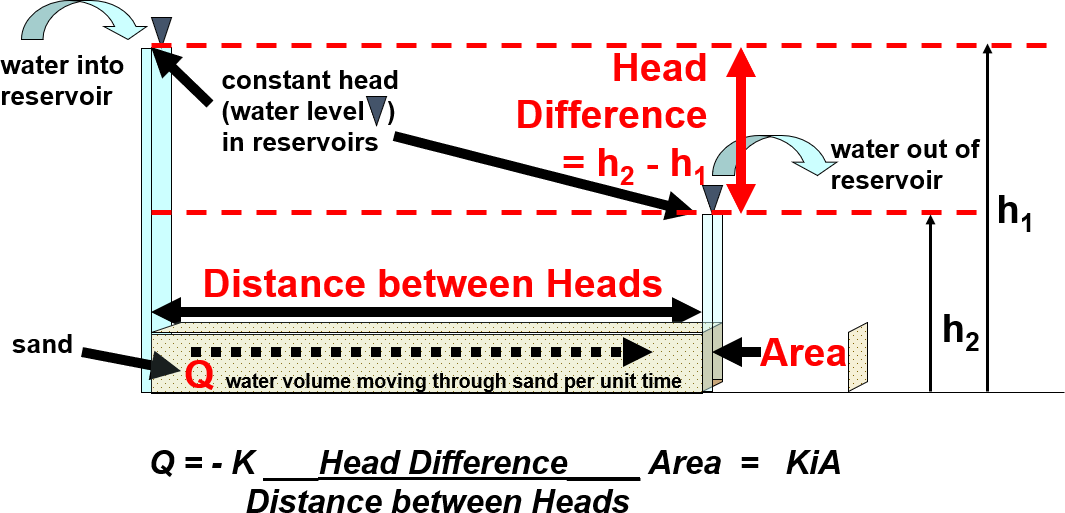
Figure Box 2-1 – Illustrated parameters of Darcy’s Law.
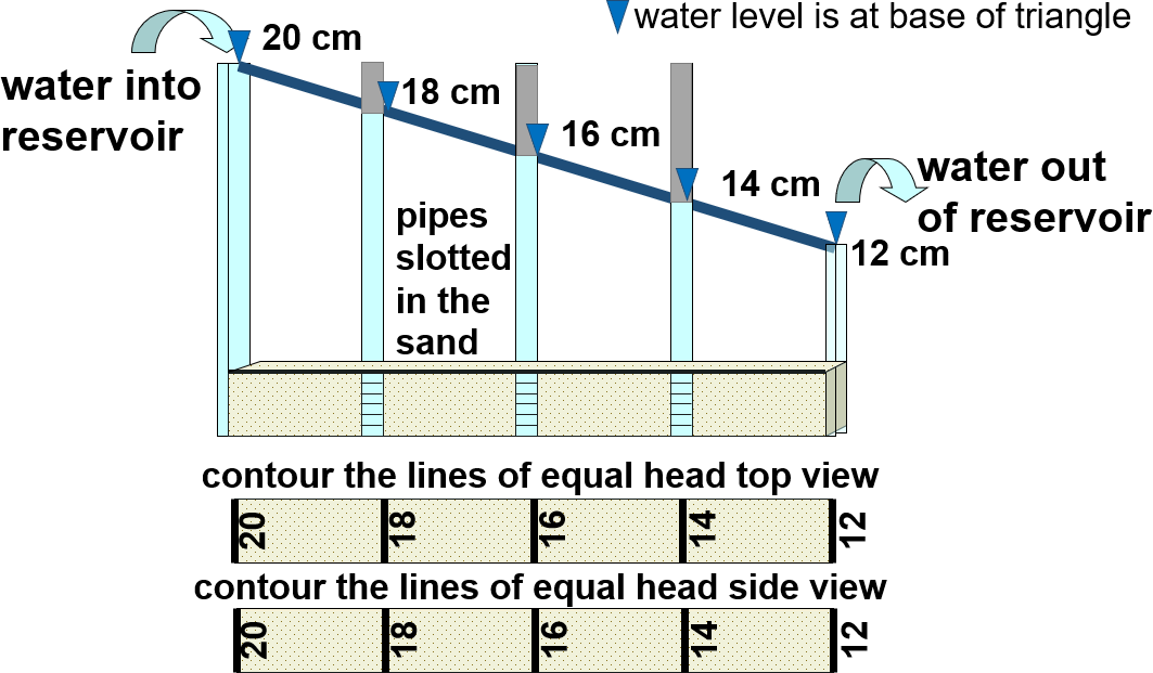
Figure Box 2-2 – According to Darcy’s Law, hydraulic head declines linearly in a homogeneous material with a constant flow area.
Specific discharge is the discharge (volumetric flow rate) divided by the flow area as shown in Equation Box 2-2. And, because the dimension of specific discharge is length over time (L/T), like the dimension for velocity, specific discharge is also referred to as Darcy velocity. However, this term can be confusing because it does not refer to the actual velocity of the groundwater (Figure Box 2-3a). Therefore, specific discharge, not Darcy velocity, is the preferred terminology used in this book.
 also it can be determined as also it can be determined as  |
(Box 2-2) |
where:
| q | = | specific discharge (L/T) |
At the microscopic scale, the detailed movements and velocities of groundwater flow in the void space between solid grains are exceedingly complex and are essentially impossible to accurately describe. However, Darcy’s Law and groundwater hydrology deal with flow at a macroscopic scale, which ignores the complex twists and turns of flow at the microscopic scale. At the macroscopic scale (the scale at which Darcy’s Law applies), we can define an “average linear groundwater velocity” as the specific discharge divided by the effective porosity, as shown in Equation Box 2-3. Effective porosity is the volume of void space that contains flowing water divided by the total volume of the porous medium (the combined volume of void space that contains flowing water and solid grains), as shown in Figure Box 2-3c. The term “linear” refers to the conceptualization that the water travels in a direct path between two points in the direction of the maximum gradient. The term “average”, however, does not refer to the average of the velocities at the microscopic scale. Instead, it is better to think of “average” as meaning “macroscopic.” To avoid writing the entire term “average linear groundwater velocity, the shorter form, “groundwater velocity”, is used in the rest of this box.
 |
(Box 2-3) |
where:
| v̅ | = | average linear groundwater velocity (L/T) |
| ne | = | effective porosity, which is the quotient of the volume of interconnected pore space and the total volume of the material (dimensionless) |
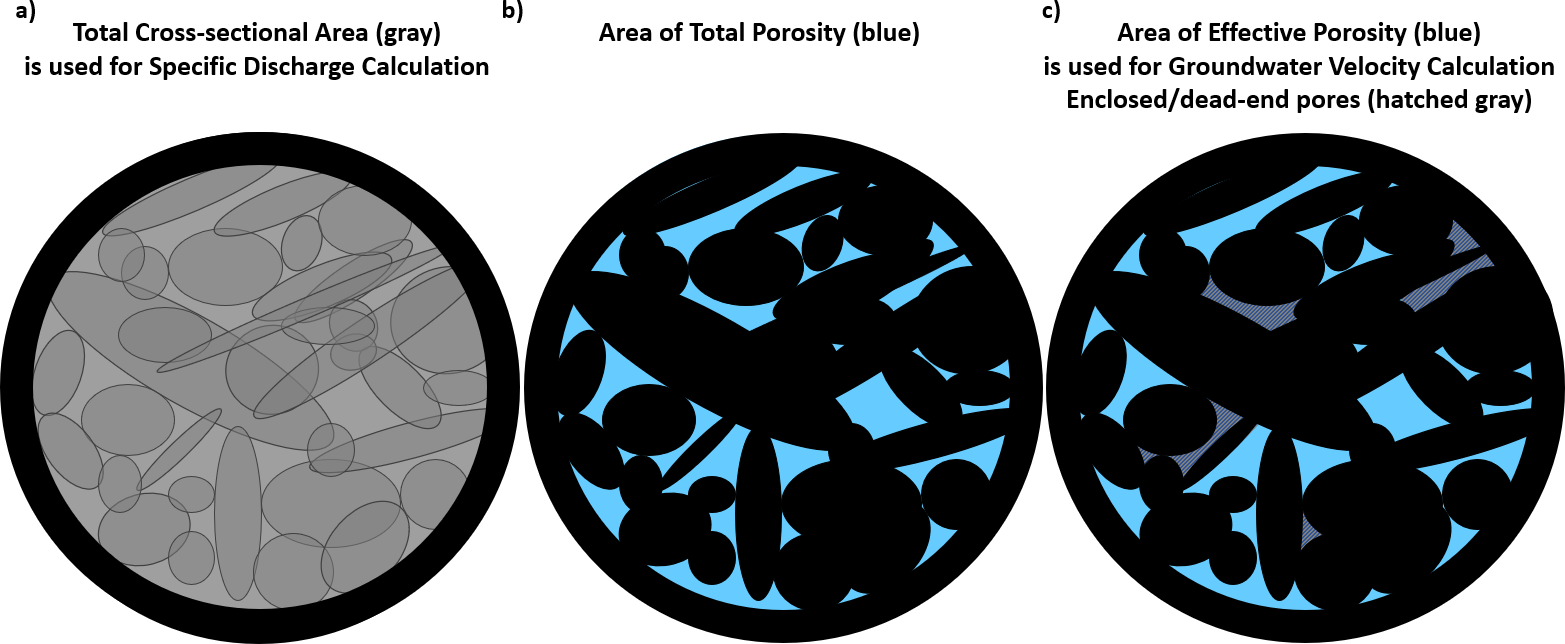
Figure Box 2-3 – Areas used to calculate specific discharge and average linear velocity: a) specific discharge is defined as the volumetric flow rate divided by the total cross-section area (shown in gray); b) porosity includes all pore spaces as shown in blue; c) average linear velocity is higher than specific discharge because it accounts for only the area of groundwater flow through connected and non-dead-end pore spaces (blue area).
When considering groundwater travel time, we use the concept of a “packet of water” to represent a small amount of water that flows together without splitting up into smaller portions. Sometimes the term “particle of water” is used to mean a packet of water. If the groundwater velocity is uniform along a flow path, the time required for a packet of water to move from one location to another along the flow path is computed by dividing the distance of travel by the groundwater velocity. This is shown in Equation Box 2-4. For a flow field with constant velocity, the travel time from point A to B is distance divide by the velocity as would be done for travel in a car. For a flow field with non-uniform groundwater velocity, calculating the travel time along a flow path from point A to point B requires dividing the flow path into small segments and computing the travel time in each segment. The total travel time from A to B is then the sum of the travel times through all the segments. In practical applications, this calculation is usually done by a computer software that tracks packets of water through a simulated groundwater flow system.
 |
(Box 2-4) |
where:
| tt | = | groundwater travel time along a flow path between two locations (T) |
| distance | = | distance along the groundwater flow path (L) |
| v̅ | = | groundwater velocity (L/T) assumed to be uniform along the flow path |