1.1 What is Graphical Construction of a Flow Net?
Graphical construction of a flow net is a method of using pencil and paper to obtain a solution to the steady-state, homogeneous, isotropic, groundwater flow equation. Steady flow is an equilibrium condition for which the hydraulic heads, flow rates and flow lines do not change with time, that is, inflow equals outflow. A flow net consists of two families of intersecting lines: equipotential lines, which connect locations of equal hydraulic head and flow lines that show paths of groundwater flow as shown in Figure 3. An impermeable dam is holding back a reservoir of water in Figure 3. Water seeps from the upstream reservoir into the underlying porous material then flows below the dam and seeps upward to the reservoir with a lower water level on the downstream side of the dam. The distribution of hydraulic head drives groundwater flow along groundwater flow lines. A brief review of hydraulic head is provided in Box 1.
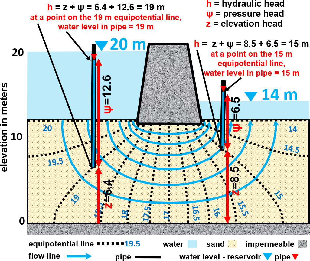
Figure 3 – A cross-sectional view of a groundwater flow net under a dam from an upper reservoir to a lower reservoir. A flow net is comprised of two sets of lines that honor Darcy’s Law and conserve mass. Equipotential lines connect points of equal hydraulic head (black dotted lines) and flow lines delineate paths of groundwater flow (blue solid arrows).
A homogeneous and isotropic groundwater system is one in which the hydraulic conductivity is the same at every location and does not vary for different directions of flow. Hydraulic conductivity is a measure of the ease with which water can pass through a material and is discussed in another Groundwater Project book (Woessner and Poeter, 2020). The groundwater flow equation is based on Darcy’s Law and conservation of mass. The groundwater flow equation is derived and discussed in another Groundwater Project book (Woessner and Poeter, 2020). A brief overview of Darcy’s Law, specific discharge, average linear groundwater velocity, and groundwater travel time are provided in Box 2 because the concepts are central to the material presented in this book.
Graphical construction of a flow net solves the two-dimensional, steady-state groundwater equation in a homogeneous and isotropic material with defined boundary conditions. Boundary conditions are discussed in another Groundwater Project book (Woessner and Poeter, 2020). Two types of boundary conditions are used in graphical construction of two-dimensional, steady-state flow nets. The flow system domain is bounded by either a constant hydraulic head boundary or a no-flow boundary. It is important to remember that “no-flow” refers to no flow across the boundary, groundwater flow occurs parallel to the boundary, such that the boundary is a flow line.
Once the geometry and boundary conditions of the system are specified, the hydraulic heads throughout the system domain can be determined; if a hydraulic conductivity is given, then the rate of flow across constant head boundaries can also be determined using Darcy’s Law and conservation of mass. The act of drawing the flow net must be done for a homogeneous and isotropic system; however, there is a procedure for scaling an anisotropic system so that an isotropic flow net can be drawn and then transformed into an anisotropic flow net. This is explained in Section 2.8 of this book. However, for cases in which the hydraulic conductivity is non-homogeneous (i.e., heterogeneous), constructing a flow net requires a numerical method using a computer.
Two requirements need to be kept in mind when drawing the equipotential and flow lines in order to obtain an accurate solution to the groundwater flow equation. First, the equipotential lines and the flow lines need to intersect at right angles. Second, the two sets of intersecting lines must form shapes with a constant aspect ratio (the same length to width ratio). The only realistic way for the human eye to achieve constant aspect ratios, is to draw “curvilinear squares”, quadrilaterals with curved sides with an aspect ratio close to 1 (Figure 3). When these two requirements are satisfied, equipotential lines will have uniform increments (contour intervals) from one line to the next, each flow tube (a region bounded by two adjacent flow lines) will carry the same volumetric flow rate (measured, for example, in cubic meters per second). An exception to these requirements may occur near the edge of the domain where a partial (or fractional) flow tube may be drawn. This exception is discussed later in this book. Finally, it is important to remember that the value of hydraulic conductivity has no influence on the head distribution in a homogeneous system, but if the hydraulic conductivity is known, then a flow net can be used to determine the volumetric flow rate through the system.
A key difference between graphical versus numerical construction of a flow net is that the graphical method requires creating both equipotential lines and flow lines, whereas the numerical method does not. Groundwater professionals commonly use a groundwater model to compute hydraulic head, then later use a flow path tracking model (also known as a particle tracking model) to compute flow lines. A project might require computing only hydraulic head, in which case flow paths are not computed.
Typically, a numerical groundwater model computes hydraulic head for a grid (or an array) of points and, unlike a graphically constructed flow net, this gives flexibility to how equipotential lines are drawn. For example, equipotential lines need not be drawn at equal increments. Flexibility also occurs in drawing flow lines. A flow path tracking model enables one to draw a flow path starting from any location. Such flexibilities mean that numerically calculated equipotential lines and flow lines do not necessarily form shapes of constant aspect ratio, and flow tubes do not necessarily carry the same volumetric flow rate. Nonetheless, these computer-generated equipotential lines and flow lines form a bona fide flow net, because they satisfy the groundwater flow equation. For example, in an aquifer with homogeneous and isotropic hydraulic conductivity, computer-generated equipotential lines cross flow lines at right angles. Numerically generated flow nets are usually used to display flow patterns rather than to compute flow rates, because flow rates are calculated by numerically solving the groundwater flow equations.
A flow net can also be constructed for two-dimensional flow in a plan view. An important assumption for graphical construction of a flow net in a plan view is the absence of areally distributed recharge, such as infiltration of precipitation to the flow system. Figure 4 illustrates a plan view of a flow net between a lake and pond in an area constrained by bedrock. If the rate of recharge is trivial relative to the volumetric lateral flow from the lake to the pond, then the flow net is a sufficiently accurate for evaluating the groundwater system.

Figure 4 – A plan view of flow in a confined aquifer penetrated by a deep lake and pond and laterally constrained by bedrock. The lake water elevation is 300 meters and the elevation of the pond surface is 200 meters. The top of the aquifer is 190 meters. Flow lines diverge on the upgradient side of the bedrock island in the middle of the aquifer and converge on the down gradient side.