4  Jacob’s Compressibility Formula for Aquifer Storage

Herbert F. Wang

4 Jacob’s Compressibility Formula for Aquifer Storage

The next major advance in the understanding of hydrogeological storage was made by C. E. Jacob (Titus, 1973) in a 1940 paper in which he linked Theis’ concept of storage as a property akin to heat capacity to Meinzer’s analysis of water stored in the Dakota aquifer as being due to aquifer compressibility. As his acknowledgment[8] makes clear, Jacob shared ideas with his colleague, C. V. Theis, at the United States Geological Society (USGS). Jacob’s goal was to derive the groundwater equivalent of the partial differential equation for time-dependent heat flow, and thereby place the mathematical description of groundwater flow on firmer physical ground than a plausible analogy.

“The writer proposes to derive “from scratch” the fundamental differential equation governing the flow of water in an elastic artesian aquifer, considering in turn each of the assumptions that are necessary to the derivation of the equation.”

Jacob computed the mass balance in a REV over a time step in which there was a change in pressure Δp. His derivation was based on three physical principles: (1) A fluid pressure decline equates to an effective increase in vertical stress. (2) A fluid pressure decline expels a water volume equal to the loss of porosity associated with aquifer compressibility. (3) A fluid pressure decline leads to volume expansion of water in the pores due to the compressibility of water itself.

The title of Meinzer’s 1928 paper called attention to the role of “compressibility and elasticity of artesian aquifers.” As evidence, he presented Terzaghi’s experiment in which a vertical stress caused porosity loss in sandstone (Figure 5). The effect of lowering pore pressure is pictured to have the same effect as an equal increase in vertical stress (Figure 8). This concept is formally stated as the “Law of Effective Stress” as shown in Equation 3.

$\displaystyle \varepsilon _{v}=\beta _{v}(\sigma _{v}-p)=\beta _{v}\sigma _{e}$

(3)

where:

β_v = ε_v/σ_v	=	vertical compressibility for p = 0 (drained conditions)
σ_e = σ_v – p	=	effective vertical stress defined to be the difference between the vertical stress and the pore pressure

The sign convention is that compressive stress is positive.

Figure showing the law of effective stress — **Figure 8 –** The law of effective stress says that the effective vertical stress *????*_e = *????*_v– p controls the vertical strain (after Atkinson, 2000).

Jacob reasoned that extraction of water from an aquifer does not change the total vertical stress. With total vertical stress constant, an increase in effective stress is equal but opposite to the decrease in fluid pressure, that is, Δ_e = –Δp, so Equation 3 becomes Equation 4.

$\displaystyle \Delta \varepsilon _{v}=-\beta _{v}\Delta p$

(4)

The sign convention is that vertical strain and vertical stress are positive in compression. Given the assumption of zero lateral strain, the vertical strain is equal to the decrease in porosity, with the caveat that the compressibility of the solid grains is negligible. In other words, Δ????_v is equal to the volume of water per unit volume of a REV that is removed from storage due to aquifer compressibility.

In addition, the expansion of the pore water volume in response to a fluid pressure decrease must be included in the water budget for a REV (Equation 5).

$\displaystyle \frac{\Delta V_{w}}{V_{w}}=-\beta _{w}\Delta p$

(5)

where:

β_w	=	Compressibility of water (4.5 × 10^-10 Pa^-1)
V_w	=	nV, where n is porosity and V is volume of the REV

By adding the two sources of water released from storage for a pore pressure decrease of -Δp, Jacob obtained an expression for coefficient of storage, S, that includes aquifer compressibility and water compressibility as well as aquifer thickness and porosity as shown in Equations 6a and 6b.

$\displaystyle S=\rho _{w}gb(\beta _{v}+n\beta _{w})$

(6a)

Dividing by aquifer thickness gives specific storage.

$\displaystyle S_{s}=\rho _{w}g(\beta _{v}+n\beta _{w})$

(6b)

The international system of units (SI) units of S_s are 1/m as indicated for Equation 2.

Jacob then obtained from mass conservation the partial differential equation for radial flow in an aquifer of thickness b that was identical in form to what Theis inferred by analogy with heat conduction. The difference was that the coefficient of storage S was expressed in terms of compressibility rather than as a quantity defined by analogy.

Terzaghi’s experiment (Figure 5 and Equation 6b) can be used to estimate the specific storage of loose sand. The vertical compressibility βv between points a and b is calculated from the slope to be 7 × 10^-10 Pa^{– 1} after converting from English units. The term nβ_w = 2 × 10^-10 Pa^-1 for a porosity of 38%. Adding the terms and multiplying by the factor ρ_wg gives a specific storage of 2.3 × 10^-4 m^-1 and the ratio of sand-to-water compressibility is 3.5. Values of specific storage are dependent on rock type as well as variability within a lithology. With those caveats, Table 2 provides order-of-magnitude values for a small set of geologic materials. The amount of water obtained for irrigation from the Dakota aquifer makes clear that large volumes of fluid can be stored in highly compressible earth materials. Nevertheless, the specific storage values in Table 2 are orders of magnitude smaller than specific yield of unconfined aquifers whose values are the aquifer porosity.

Table 2 – Rock compressibility and specific storage of a few geologic materials (Palciauskas and Domenico, 1989). The rock compressibility and specific storage values are for isotropic confining stress, not vertical stress. The values come from a variety of sources. The limestone measurements are for barometric or tidal loadings. The other values came from handbooks and were calculated with assumptions. Specific storage in terms of head was computed from its value in terms of pressure using ρ_w = 1000 kg/m³ and g = 9.8 m/s². For comparison, compressibility of water β_w = 4.5 × 10^-10 Pa^-1.

Geologic material	Rock compressibility	Specific storage in terms of pressure	Specific storage in terms of head
	β, 10^-10 Pa^-1	S_s/(ρ_wg), 10^-10 Pa^-1	S_s, 10^-6 m^-1
Clay	160	162	159
Mudstone	4.6	5.4	5.3
Kayenta Sandstone	1.1	1.2	1.2
Limestone	0.3	0.95	0.93
Hanford Basalt	0.22	0.44	0.43

In hydrogeology, aquifer compressibility is typically more significant than water compressibility. On the other hand, petroleum engineers generally considered oil reservoirs to be incompressible because they are at greater depth. Jacob examined this assumption for the East Texas oilfield described by Muskat (1937) in his classic treatise Flow of Homogeneous Fluids through Porous Media. The field produced 500 million barrels (80 million m³) of oil with a pressure drop of 375 psi (2.6 MPa). By assuming a rigid reservoir, Muskat required that the oil in place had to contain sufficient dissolved gas to increase the fluid compressibility by a factor of 20 in order to produce this quantity from fluid compressibility alone, even though the oil was undersaturated. Jacob suggested instead that compressibility of the reservoir’s Woodbine sand and associated clay beds would more likely account for the production.

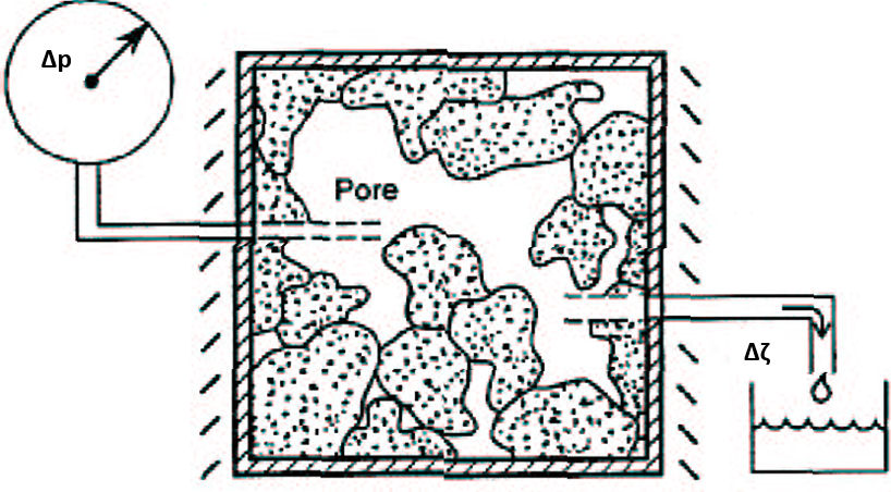
It should be emphasized that the storage coefficients S and S_s in Equation 6a or 6b can be measured directly in the field from a pumping test or in the laboratory by adhering to its definition as the ratio of water volume removed from storage due to pore pressure change (Figure 9). However, this direct measurement is difficult to perform accurately because fluid storage in tubing connected to the rock sample’s pore volume must be included in the accounting.

Figure showing measurement of specific storage — **Figure 9 –** Measurement of specific storage in terms of change in fluid pressure Equation 2b (Wang, 2000).

In addition to Equation 6a, Jacob derived equations for the water-level response to aquifer loading by water tides or changes in barometric pressure, also in terms of aquifer and water compressibility, which could provide an indirect measurement of coefficient of storage. The assumed large horizontal extent of the loading induces a fluid pressure in the aquifer because the fluid cannot escape as it is being loaded. In soil mechanics, the aquifer is said to be undrained. In tidal or barometric loading, the vertical stress is decidedly not constant. Water can be added to or removed from storage when vertical stress is applied in addition to when pore pressure changes (compare with Equation 2b). Therefore, in general, the increment of fluid content must be expressed in terms of changes in both vertical stress and pore pressure. The simplest form for an equation is to consider increment of fluid content to be a linear function of both variables.

$\displaystyle \zeta =-\beta _{v}\Delta \sigma _{v}+\rho _{w}gS_{s}\Delta p$

(7a)

The sign convention is that is positive when water is added to the REV and Δσ_v is positive when the REV is compressed. The first term on the right in Equation 7a is the increment of fluid content associated with a change in vertical stress when there is no change in fluid pressure. Jacob made the assumption that the volume of water in storage in a REV decreases by the same amount as does the volume of the REV itself, that is, the change of water in storage is the negative of the strain, which is why the coefficient of Δσ_v in Equation 7a is β_v. The second term on the right in Equation 7a is the increment of fluid content associated with a change in fluid pressure when there is no change in vertical stress, which is precisely the definition of specific storage (compare with Equation 2).

Equation 7a is one of two basic constitutive equations of poroelasticity for the special case of areally extensive, vertical loading (Wang, 2000). The other constitutive equation linearly relates vertical strain to changes in vertical stress and pore pressure.

$\displaystyle \Delta \varepsilon _{v} =\beta _{v}\Delta \sigma _{v}-\beta _{v}\Delta p$

(7b)

Equation 7b gives the vertical strain as the sum of two terms. The first term states that the vertical strain is the vertical strain due to a change in vertical stress when there is no change in fluid pressure and the second term is the vertical strain associated with a change in fluid pressure when there is no change in vertical stress. The coefficient of proportionality is β_v for both terms by the law of effective stress, i.e., Equation 7b is simply a restatement of Equation 3.

The in-phase response of water levels in an aquifer to ocean tides (Figure 6) was cited by Meinzer as evidence of aquifer elasticity. The ratio of the increase in water level in a well to the increase in ocean level, is called tidal efficiency, T.E. This ratio is equal to the ratio of Δp/Δσ_v. Assuming no water enters or leaves the aquifer by virtue of the large areal extent of the loading and inserting the undrained condition, ζ = 0, in Equation 7a gives the undrained pore pressure response to be Δp = β_vσ_v/(ρ_wgS_s). Then substituting Equation 6b for S_s yields Equation 8.

$\displaystyle T.E.=\frac{\beta _{v}}{\beta _{v}+n\beta _{w}}$

(8)

Barometric efficiency, B.E., is similarly defined to be the ratio of the increase in water level to the increase in vertical stress (expressed as an equivalent head increase). A difference from the tidal efficiency in terms of well response is that a change ∆p in atmospheric pressure directly changes the water level in the well by -Δp/ρ_wg. This must be added to the amount induced in the aquifer by the atmosphere loading as in the tidal loading case. Thus, B.E. = 1 – T.E. and can be expressed as Equation 9.

$\displaystyle B.E.=\frac{n\beta _{w}}{\beta _{v}+n\beta _{w}}$

(9)

The expressions for tidal efficiency and barometric efficiency contain the same aquifer properties as specific storage, that is, vertical compressibility, water compressibility, and porosity. Measuring T.E. or B.E. and assuming n and β_w to be knowns means that β_v, and hence, S_s can be obtained from Equation 8 or 9 and the ratio of the contribution from water compressibility, nβ_w, to aquifer compressibility, β_v, can be calculated.

Jacob (1941) used tidal efficiency to compute indirectly the coefficient of storage because it was more easily determined than the barometric efficiency. He compared the relative contributions of aquifer elasticity and water compressibility from tidal responses (e.g., Figure 6) with those from pumping tests at depths between 715 and 800 ft in the Lloyd sand on Long Island of the United States. The ratio of aquifer compressibility to water compressibility obtained from tidal efficiency was 1.7 whereas it was 2.8 from pumping test analysis.

[8] “The writer is greatly indebted to his colleagues in the Geological Survey for timely suggestions and criticism, and especially to C. V. Theis, as many of the ideas expressed herein have been taken from his personal communications to the writer.”

License