1.1 Measurement Physics: The Relation between Data (Voltage Differences) and Parameters (Electrical Conductivity or Chargeability)
ER data acquisition systems drive an electric current that can range from milliamps (mA) to several amps into the subsurface through galvanic contact. Current is injected between two electrodes, a positive and a negative one (the current electrodes), and the resultant electric potential (specifically, the voltage difference) is measured between two or more additional electrodes (the potential electrodes, see Figure 1.). The physics is mathematically analogous to a two-well pumping test, where water is injected in one well and removed from another, and the resultant head difference at steady-state would be measured between two other locations. This four-electrode injection/measurement procedure is repeated for as many combinations of current and potential electrode positions as desired, and usually involves the acquisition of many hundreds or thousands of multi-electrode combinations.

Figure 1 – Example of ER data collection. Multiple electrodes are installed along the ground surface (or in boreholes), and two electrodes at a time are used to drive current into the subsurface. The resulting voltage difference is measured between two or more potential electrodes. Flow and equipotential lines are analogous to those estimated from the groundwater flow equation, where current and fluid flux are mathematically parallel, as are voltages and heads, which are both potentials.
The measurements presented by ER instrumentation are voltage differences in volts (equivalent to differences in hydraulic heads in the analogy to groundwater flow), which are divided by the applied current to calculate resistance values (from Ohm’s law, where R = ∆V/I) in ohm (Ω), sometimes referred to as transfer resistance. The physical measurement of resistance is not an intrinsic property of a material (in our case rock or soil) because it depends on the geometry of, or distance between, electrodes used for measurement. A well-known example is the resistance of a length of wire. The resistance across 100 m of homogeneous copper wire would be 100 times the resistance across 1 m of the same wire. The wire has an intrinsic resistivity (in this case, the resistivity would be very low or the conductivity very high as copper is an excellent conductor) that limits current flow as evident from an observed voltage drop. Thus, in ER we measure a resistance that must be converted to a relevant intrinsic property, electrical resistivity, ρ (or its reciprocal, electrical conductivity, σ), from knowledge of the electrode locations. In the flow analogy, hydraulic conductivity is treated as an intrinsic property, whereas transmissivity is a function of geometry. In SI units, resistivity has units of ohm-meter (Ω-m) and conductivity has units of Siemens/meter (S/m). Each measured resistance is a function of the electrode locations, as noted above, and the electrical properties of both solids and liquids in the system.
The physics underlying ER measurements are described by the Poisson equation (Equation 1), which is a simplification of the Maxwell equations. This is also the equation that describes steady-state groundwater flow.
| ∇·σ(x, y, z)∇V(x, y, z) = −Iδ(x − xs, y − ys, z − zs) | (1) |
subject to boundary conditions, where:
| ∇ | = | Gradient operator |
| ∇· | = | Divergence operator |
| σ | = | Electrical conductivity, an intrinsic property of the material (Siemens/meter) |
| V | = | Electric potential (Volts), where V can be used to determine the voltage differences between two potential electrodes for a given current injection |
| I | = | Electric current source magnitude, otherwise known as the current injected in the field (Amperes) |
| δ | = | Dirac delta function |
| x, y, z | = | Spatial position vectors (meters) |
| xs, ys, zs | = | Spatial coordinates of the current source (meters) |
As with the groundwater flow equation, Equation 1 can be simplified to an equation for two-dimensional (2-D) systems, and/or to an equation where the electrical conductivity is considered to be homogeneous and isotropic (see Section 7 of the Groundwater Project book “Hydrogeologic Properties of Earth Materials and Principles of Groundwater Flow”). 3-D data acquisition and inversion methods are increasingly practical and appropriate, although many practitioners still use 2-D inversion. Commonly, commercially available software for 2-D inversion invokes what is known as a 2.5-D assumption for computational efficiency. Under this assumption, inverse modeling is performed for a 2-D parameterization (e.g., to identify the best-fit cross section), while forward modeling of the electrical measurements is performed in 3-D. The 2-D structure is assumed to extend infinitely into the third dimension (e.g., Dey and Morrison, 1979; LaBrecque et al., 1996; see Section 4.2 for more details). The 2.5-D approximation thus combines a 2-D parameterization with 3-D physics. Conceptually this is similar to classical pumping test analysis, where hydrogeologists combine a 1-D parameterization (layers) and 2-D (axisymmetric) flow.
Equation 1 combines conservation of charge and Ohm’s law. Ohm’s law, shown in continuous form by Equation 2, is the constitutive relation analogous to Darcy’s law, linking electrical (as opposed to hydraulic) potential gradients and fluxes.
| j = −σ∇V | (2) |
In geophysics, this link is assumed to be linear. Here, j is the electric current density (Amperes/m2) in the ground in response to the external current source (I) and is analogous to the specific discharge in Darcy’s Law. In adopting Equation 1, we make some important assumptions about our measurement. Equation 1 assumes equilibrium or steady-state electrical conditions and includes neither transient (i.e., induced polarization) effects nor current sources other than what is injected through the current electrodes (e.g., no spontaneous potentials), which are assumed to act at a single point (i.e., xs, ys, zs). The validity of these assumptions depends in part on instrument settings, as explained in Section 3, below. Equations 1 and 2 describe the link between the subsurface potential distribution (V), which determines the voltage differences between two potential electrodes (∆V), the current injection magnitude and location, and the electrical conductivity (σ).
In some software packages, the data are specified in terms of resistance (∆V/I) where both I and ∆V are reported by the instrumentation. Other packages expect data in the form of apparent resistivity, ρa, which is the resistivity that the subsurface would have if it were homogeneous and isotropic and is calculated as shown in Equation 3.
| ρa = Kg(ΔV/I) | (3) |
Kg is a geometric factor (in meters) accounting for electrode configuration. In our earlier example of the copper wire, this geometric factor is simply the cross-sectional area of the wire divided by its length. Apparent resistivity is sometimes preferred over resistance because it scales the data to have the same units and magnitude as the intrinsic property being estimated (electrical resistivity), and thus it is more intuitive. Note that the resistance measurements can be both positive and negative, as geometric factors can be positive or negative. It is important to note that intrinsic subsurface electrical conductivity cannot be negative, and neither are the magnitudes of injected currents. However, the sign of the measured potential difference is purely dependent on which electrode we use as our reference electrode, and thus negative voltages (and resistances) can be recorded. Although the apparent resistivity is typically positive, negative apparent resistivities are also possible. A measurement that would be positive under homogeneous subsurface conditions may be negative under certain heterogeneous subsurface conditions (e.g., Wilkinson et al., 2008; Jung et al., 2009). For this reason, it is crucial to collect signed voltage differences in the field, rather than the absolute value of the voltage difference between electrodes. The use of apparent resistivity can be helpful in assessing measurement errors when compared to examining resistance values, given that the apparent resistivity values are of similar magnitude to one another. In the field, geophysicists used to plot pseudosections of apparent resistivity, which assign the volumetric measurements to a point location in x–z space based on the measurement-electrode locations (e.g., Hallof, 1957); these plots are still generated by many inversion programs. In general, plotting measurements prior to inversion is important for visualizing trends that may be indicative of certain subsurface objects or to identify obvious errors as in the case of malfunctioning electrodes.
Induced polarization measurements record the effect of temporary charge storage on the electric field. One way to observe storage effects is to capture the transient voltage decay that occurs on abrupt termination of the applied electric current when the Earth stores charge. This time–domain IP effect is quantified as an integral of Vm, the voltage decay curve, from t1 to t2 divided by the primary or total voltage (VT) as shown by Equation 4 and in Figure 2a.
| [latex]\displaystyle M_{a}=\frac{1}{(t_{2}-t_{1})}\frac{\int_{t_{1}}^{t_{2}}V_{m}}{V_{T}}[/latex] | (4) |
Ma is the apparent chargeability. Similar to apparent resistivity, the apparent chargeability depends on the electrode locations and is different from the intrinsic chargeability of the subsurface, which describes the polarization strength of a geologic material. It is worth noting also that sampling period is not standard between different instruments and may affect measurements; thus, instrument settings must be consistent to allow for meaningful comparisons of measurements between surveys. A number of conventions have been proposed, e.g., integration over one log cycle or a specified time window (Sumner, 1976). Apparent and intrinsic chargeability are both unitless although typically expressed as mV/V.
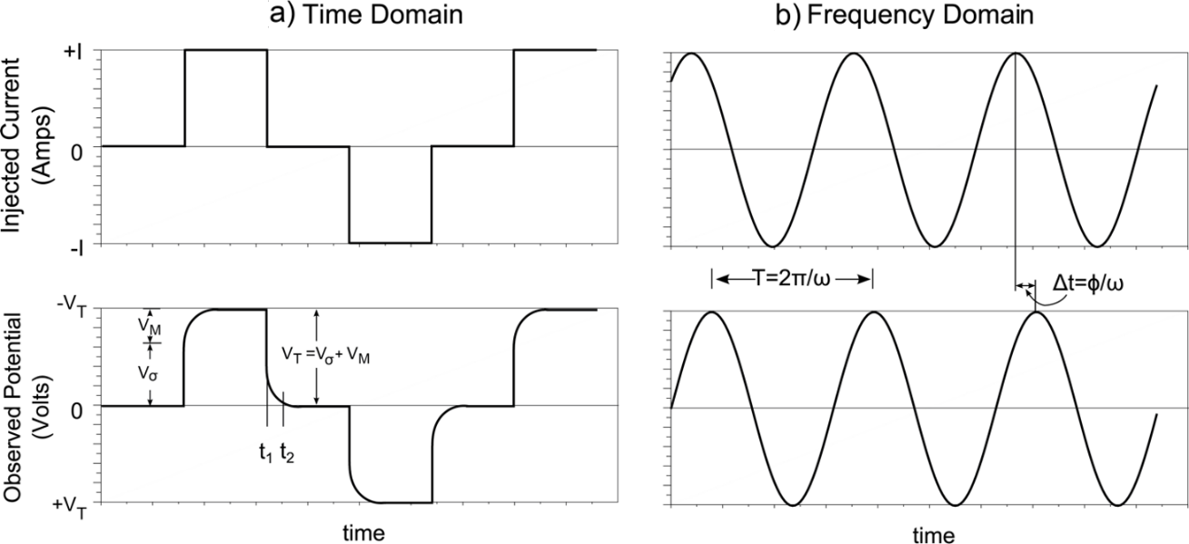
Figure 2 – Different ways to measure induced polarization: a) a time-domain measurement, where voltage decay is recorded following abrupt current termination, and b) a frequency-domain measurement, where magnitude and phase of a sinusoidal voltage with a period T (related to frequency ω recorded between two electrodes lags behind the current recorded across a reference resistor placed in series with the Earth by a time ∆t. Note that in ER measurements, voltages are only measured at the plateau of the injected current (i.e., VT), not during the decay.
The intrinsic chargeability or phase of the Earth must be positive. However, the measured apparent chargeability or measured apparent phase over a heterogenous Earth can be positive or negative, depending on the location of chargeable objects relative to the sensitivity pattern of the electrode array, described in more detail below. Any array will have some regions of negative sensitivity, where in ER, an increase in subsurface resistivity will counterintuitively be observed as a decrease in measured resistance. When a highly chargeable object is located within this region of negative sensitivity, a negative apparent chargeability can be recorded with IP (Dahlin and Loke, 2015). When expressed with respect to a complex impedance or complex resistivity, the phase should normally be negative, being consistent with Figure 2 where the voltage lags in time behind the current waveform. However, the measured apparent phase recorded over a heterogeneous Earth can sometimes be positive (Luo and Zhang, 1998; Wang et al., 2020) as a result of the sensitivity patterns of an array. A practitioner may be tempted to discard negative apparent chargeabilities or positive (for complex impedance or resistivity) apparent phase as data errors. Error checks, described in Section 3.3, can help to differentiate between errors and negative apparent chargeabilities that inform on the subsurface structure.
The physics of induced polarization can be incorporated into Equation 1 by representing the conductivity and potential gradient terms as complex numbers, as shown in Equation 5.
| ∇·σ*(x, y, z)∇V*(x, y, z) = −Iδ(x − xs, y − ys, z − zs) | (5) |
Here, σ* is known as the complex conductivity. The real and imaginary components of the complex conductivity separate out the electrical conduction and polarization properties of the subsurface. In the mathematical analogy to groundwater flow, chargeability is related to parameters controlling storage (e.g., specific storage or storativity), and Equation 5 resembles the transient groundwater flow equation with a single complex-valued parameter, σ*, where the real part relates to resistance (or its reciprocal, conductance) and the imaginary part to reactance (or its reciprocal, susceptance). Indeed, the electrical analogy for the transient problem was the basis for simulating non-equilibrium groundwater flow using resistor-capacitor networks prior to the advent of digital computing (Freeze and Cherry, 1979).
Frequency–domain IP considers measurements in terms of the frequency of waveforms ( Figure 2b), which are made by using a sine-wave current source, and measuring the magnitude and phase (Ø) of the complex resistance (ΔV/I)* or of the complex apparent resistivity ρa*. The phase refers to the phase shift between the injected current and the measured voltage and is the frequency-domain measure of the IP effect. In the absence of current storage (either in non-polarizing materials or because we do not measure the time-varying piece), Ø = 0 and Equation 5 simplifies to Equation 1. Frequency-domain measurements are popular in the laboratory, and some instruments exist to perform field-scale frequency-domain acquisition. However, it is often simpler to measure the field IP effect using time–domain IP ( Figure 2a). The time-domain and frequency-domain IP effects are theoretically equivalent, and one can be determined from the other through a Fourier transformation (the Fourier transform of a time series is a complex valued function of frequency).
Regardless of whether IP data are being collected, the goal of data collection is to create a cross section or volume distribution of subsurface electrical conductivity in x–y (or x–y–z) space, which requires the process of inversion, described in detail in Section 4. Inversion software solves the forward model problem using Equation 1 or 5, which takes assumed model parameters (electrical conductivity or resistivity and chargeability or phase) and produces model predictions that can be compared with observed data—resistances or apparent resistivity and apparent chargeability or apparent phase. ER inversion is commonly done using finite-difference or finite-element techniques for solving partial differential equations, where Equation 1 (or Equation 5 in the case of IP) is solved at spatially distributed discrete locations corresponding to the centers of finite-difference grid cells or to nodes in a finite-element mesh, with the accuracy of the solution depending on the level of discretization, as outlined in Section 2.2. Finite-difference codes are not frequently seen for surface data collection due to complexities with topography. Depending on the survey geometry (i.e., number and placement of electrodes), inversion can produce 1-, 2- or 3-D tomograms, reconstructed images that show the estimated subsurface distribution of electrical resistivity or conductivity. The term tomography refers to the image reconstruction process using ER measurements and is described in Section 4.