2.1 Geometric Factors
We introduced the concept of the geometric factor (Equation 3) as the parameter that converts a measured resistance to apparent resistivity. For surface arrays, the underlying math to calculate the geometric factor is fairly simple. Assuming a homogeneous and isotropic half space (meaning the same electrical conductivity in the earth to infinite distance below a surface boundary) without any electrical sources, the geometric factor Kg for every quadripole can be calculated for surface arrays using Equation 6a.
| [latex]\displaystyle K_{g}=\frac{2\pi }{\left [\frac{1}{\overline{AM}}-\frac{1}{\overline{AN}}-\frac{1}{\overline{BM}}+\frac{1}{\overline{BN}} \right]}[/latex] | (6a) |
[latex]\overline{AM}[/latex], [latex]\overline{AN}[/latex], [latex]\overline{BM}[/latex], and [latex]\overline{BN}[/latex] are the distances between electrodes A and M, A and N, B and M, and B and N, respectively. Current electrodes are defined as A and B and potential electrodes are M and N. Current electrodes are defined as A and B and potential electrodes are M and N (Figure 5). These electrodes are often also called C+, C−, P+, and P−, respectively, in other literature, however the older A, B, M, N standard is used in this book. The geometric factor accounts for the arrangement of electrodes and allows one to calculate an apparent resistivity (Equation 3).
For borehole geometries, the electrodes are located within the half-space rather than at the boundary at the Earth’s surface. In this case, use of Equation 6a is inappropriate, as it does not account for the no-flow boundary at Earth’s surface. To account for the effect of the boundary on cross-well measurements, the method of images from optics is invoked. This approach is analogous to the use of image wells in groundwater hydrology for analytical modeling of aquifer response to pumping. Here, imaginary image current electrodes are introduced on the other side of the boundary, equidistant from the real current electrodes, to mathematically produce a no-flow condition at the Earth’s surface and calculate a geometric factor for borehole arrays as shown in Equation 6b.
| [latex]\displaystyle K_{g}=\frac{4\pi }{\left [\frac{1}{\overline{AM}}+\frac{1}{\overline{A_{image}M}}-\frac{1}{\overline{AN}}-\frac{1}{\overline{A_{image}N}}-\frac{1}{\overline{BM}}-\frac{1}{\overline{B_{image}M}}+\frac{1}{\overline{BN}}+\frac{1}{\overline{B_{image}N}} \right]}[/latex] | (6b) |
Here, “image” indicates the image current electrode. When the electrodes are all on the boundary, Equation 6b simplifies to Equation 6a. Also, limited burial is necessary before Equation 6b simplifies to twice the result of Equation 6a, as the distances from the potential electrodes to the true current electrodes and their images are approximately equal.
Quadripoles with large geometric factors may produce small voltage differences, which are prone to measurement errors due to a lower signal-to-noise ratio. These are manifest (via propagation of errors) as higher relative errors in apparent resistivity data. A critical geometric-factor cutoff can be determined based on the average expected electrical conductivity of the subsurface and the instrument specifications. Based on Equation 3, for a given geometric factor and expected instrument error (in terms of voltage, inserted as the potential difference), we can calculate the expected error in apparent resistivity. Figure 6 illustrates how error in measured potential difference translates into error in calculated apparent resistivity as a function of Kg. In this example, we consider an applied current of 50 mA and assume a 1-microvolt (μV) instrument accuracy (note the logarithmic scale). In practice, accuracy may be less. As evident in Figure 6, for large geometric factors or small assumed apparent resistivity, errors are larger relative to measurements.
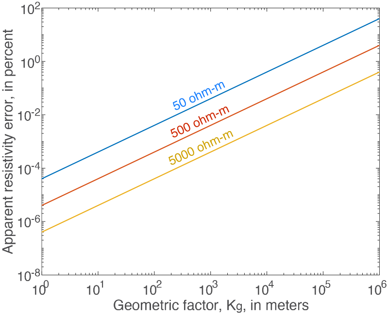
Figure 6 – Apparent resistivity error, as a percentage of the true apparent resistivity, as a function of geometric factor for three different values of resistivity (50, 500, and 5,000 Ω-m), assuming the voltage accuracy is 1 microvolt and the applied current is 50 milliamperes, where apparent resistivity error is given by Kg*Verror/I, which is then compared to the assumed apparent resistivity in a relative sense. An error in the measured voltage translates into error in calculated apparent resistivity as a function of Kg. In practice, larger errors may occur in the field.