4.1 The Goal of Inversion

Once electrical imaging data are collected, they are inverted to obtain a spatially discretized (i.e., gridded or meshed) distribution of the electrical properties of the subsurface. In the case of ER measurements alone, it is just the electrical conductivity structure that is estimated by the inversion. When IP datasets are acquired, both the electrical conductivity and the intrinsic chargeability (or the intrinsic phase) structure are estimated, and IP data cannot be inverted without ER data. With IP datasets, images can be presented in terms of the real and imaginary components of the complex conductivity. Irrespective of what data have been acquired—whether ER data alone, or ER and IP data combined—the inversion of electrical imaging datasets involves a number of common key steps/concepts. For simplicity, we describe the inversion process from the perspective of an ER dataset alone, but the mechanics and considerations introduced in this section apply equally to combined ER and IP datasets.

The goal of inversion of an ER dataset is to recover a subsurface distribution of electrical conductivity (Figure 10), σ_x,y,z (note for frequency domain, IP this would be σ*_x,y,z) that could have produced the observed data (step 2 and 3 below). The general procedure for inverse modeling consists of the following steps:

1. Start with a distribution of electrical conductivity (typically a homogeneous starting model corresponding to the average apparent conductivity measured in the field);
2. Use a forward simulator which, for the given distribution of electrical conductivity, calculates predicted data using Equation 1 (or Equation 5 for frequency-domain IP, and time-domain IP with caveats as noted below);
3. Calculate the misfit between the predicted and the observed data and also a measure of the complexity (e.g., roughness) of the electrical conductivity distribution; and
4. If the misfit is less than our stopping criteria, stop and accept the current subsurface distribution of electrical conductivity as the final result. If not, modify the model to improve the fit, and return to step 2.

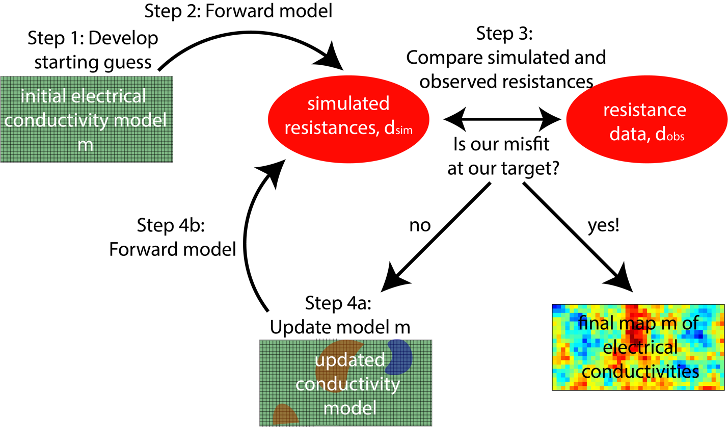
Figure 10 – A simplified overview of the inversion process.

In inversion codes, forward models are called repeatedly within an optimization framework to calculate predicted data for comparison with observed data. The optimization iteratively updates the model to improve the match between predictions and observations. Data processing and inversion can be performed with commercially available software packages such as AGI EarthImager (LaBrecque and Yang, 2001), Res2DInv (Loke and Barker, 1996), or MPT ERTLab, and public-domain or freeware packages such as RESINVM3D (Pidlisecky et al., 2007), E4D (Johnson et al., 2010), ResIPy (Blanchy et al., 2020), pyGIMLIi (Rucker et al., 2017), or SimPEG (Cockett et al., 2015). The majority of these codes also permit the inversion of IP datasets. It is not our goal to review or compare these codes, but most follow similar inversion approaches, which are based on Gauss-Newton, quasi-Newton or steepest-descent algorithms (Tarantola, 1987), with some codes supporting use of multiple inversion algorithms. Depending on selection of modeling and inversion parameters, these codes generally can be made to produce similar results. Default values differ greatly, however, and it is not always clear how parameters are used within the inversion. Selection of many inversion settings can be somewhat subjective and should be guided by prior knowledge of the site geology or the nature of the targets. For example, in a layered system, one might choose to apply anisotropic smoothing, which will result in a tomogram that has a layered character. For results to be reproducible, it is critical to (1) report all parameter selections including default values, (2) document the algorithm used by the software, and (3) archive a copy of the software code or executable. Justifications of parameter choices should also be documented. An example of how inversion settings affect tomograms is demonstrated in Section 5.2. The process for selecting inversion settings should be guided by prior information, and many hydrogeologists will find it useful to work with a geophysicist while learning inverse techniques for these data.

Ideally, the inversion should result in the true distribution of electrical conductivities of the subsurface. In practice, this is impossible for several reasons. First, the electrical conductivity estimates are commonly produced for blocks with dimensions of tens of centimeters to several meters on the side, while earth conductivity varies on much smaller scales. Thus, the best one can hope for is to identify block conductivities that represent some sort of weighted, spatial averages. Additionally, there commonly is not enough information in the data to uniquely determine all the block bulk conductivity parameter values. Unlike medical imaging, where it is possible to acquire a 360-degree view around the target, ER is usually limited to surface and borehole electrodes unless working on soil cores or experimental tanks, which is partly why medical imaging offers higher resolution compared to geophysical imaging. The result of this limited available information is called ill–conditioning, which is a property of matrix-inversion problems where limited data sensitivity to parameter values causes uncertainties in the data (e.g., resistance measurements) and can lead to large errors in the parameter estimates (e.g., electrical conductivity values). This ill conditioning is typically rectified through model regularization, which imposes additional constraints on the estimated model to get a unique set of stable solutions, as described subsequently. Additionally, as noted above, depending on the discretization of the finite-difference grid or finite-element mesh used for numerical approximations of Equation 1 or 5, some quadripoles may model poorly. For example, the inverse model would not be able to accurately match these data. Finally, accurate representation of data errors (for example using reciprocal measurements or stacking described above) is needed to ensure quality inversion results that do not over- or under-fit measurements.

Resistivity software packages that incorporate time-domain IP measurements model the distribution of the intrinsic chargeability in addition to electrical conductivity. In contrast, frequency-domain measurements are processed with algorithms that model the complex electrical conductivity distribution per Equation 5. The electrical conductivity magnitude and phase, or the real and imaginary parts of the complex electrical conductivity, can be imaged. The measured apparent chargeability and measured apparent phase are directly proportional to each other, although the proportionality constant will vary depending on how a time-domain instrument is configured (Slater and Lesmes, 2002). Consequently, time-domain measurements can be modeled using Equation 5 if this proportionality constant is defined (Mwakanyamale et al., 2012).