6.1 Case Study 1: Hypothetical Stream-Aquifer System
Description of Problem
When a hypothetical system is stressed in a simulation model, the responses can be analyzed and interpreted without the uncertainty normally associated with complex field systems. Furthermore, additional factors or complexities can be added in individual increments, thereby simplifying the analysis of cause and effect. Thus, the links and relations between stresses and responses (causes and effects) can be more clearly and definitively identified.
For this purpose, we identify a hypothetical desert basin with a perennial stream along one edge of the valley, based on one designed and used by Barlow and Leake (2012) to illustrate the effects of pumping on streamflow. We modify their example problem, similarly to the modifications of Konikow and Leake (2014), to illustrate additional effects of pumping a well on the hydrology of such a stream-aquifer system (Figure 17). Among other changes, we add more realistic and variable land-surface elevations that will induce spatially varying evapotranspiration (ET) losses, which vary as a function of the depth to the water table. ET consists of both direct evaporation from the water table surface and transpiration by plants. Substantial groundwater use by phreatophytes is evidenced by diurnal fluctuations of the water table (e.g., Butler et al., 2007). Groundwater evaporation is greatest when the water table is at or very close to the land surface. As the water table becomes deeper, the transport distance for water vapor between the water table and the atmosphere increases and dissipation of humidity in the soil is hindered, hence the evaporative flux from the saturated zone decreases. Transpiration is generally the larger component of ET. As the depth to the water table increases, the percentage of plant roots that are sufficiently long and deep to penetrate the water table tends to decrease, and the greater the energy requirement needed to lift water over the larger distance to the land surface. At some point, the water table may be so deep that no roots can reach it.
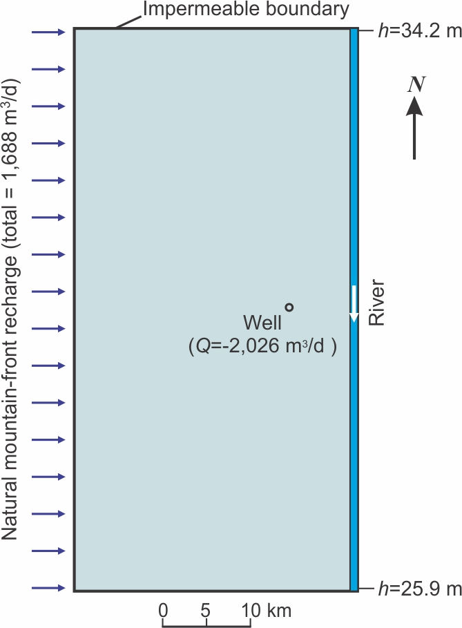
The hypothetical aquifer is 32.2 km (20 mi) wide by 64.4 km (40 mi) long, with a total area of 2,072 km2 (800 mi2). The river is in good hydraulic connection with the alluvial aquifer; the specified flow into the upstream end of the river is 20,000 m3/d. It is assumed, for simplicity, that there is neither direct precipitation on the river nor evaporation from the river, and that the inflow to the upstream end of the river is constant. Mountain front recharge totaling 1,688 m3/d is uniformly distributed along the western boundary of the basin. The hydraulic conductivity of the aquifer is 15.2 m/d and its thickness averages about 150 m, which is much smaller than its lateral extent. The specific yield is 0.20. The rectangular aquifer is surrounded by impermeable boundaries, including along the distal side of the river. There is one fully penetrating well located near the center of the system, at a distance of 8.05 km (5 mi) from the river. It pumps at a rate of 2,026 m3/d (0.83 ft3/s).
The land surface is represented as having three terrace levels above the river (Figure 18). The elevation differences between adjacent terraces is about 1 m, with the highest elevations being the furthest from the river. Note that the land-surface elevation is not assumed to coincide with either the streambed elevation or the water surface in the river. Rather, the head in the river is assumed to vary linearly between the upstream and downstream heads shown in Figure 17 and to remain constant in time.

Simulation Model
A two-dimensional numerical model was developed to simulate transient groundwater flow in this system. The model was developed using the MODFLOW-NWT code, (Niswonger et al., 2011). Streamflow was represented using the Streamflow Routing Package (SFR2) (Niswonger and Prudic, 2005). The model domain was discretized into 80 rows and 40 columns of square cells within a single model layer. The grid spacing was 805 m in each direction. Layer thickness varied depending on the water-table position. For simplification in the model, it was assumed that the streambed elevation can be specified as the linearly varying river heads shown in Figure 17 and that the water depth would remain constant and uniform at 0.001 m.
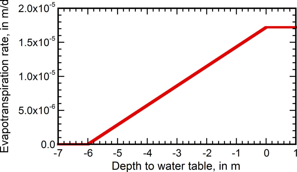
In the model, evapotranspiration (ET) is assumed to vary as a linear function of the depth to the water table (Figure 19). The ET Surface is the water-table elevation at which the maximum value of evapotranspiration loss occurs (assumed to coincide with the land surface). The extinction depth (or cutoff depth) is that depth of water table at which ET no longer occurs. The ET rate varies linearly between those two limits.

Base Case: No Recharge and No ET (No Phreatophytes)
To develop a “base case” for assessing the effects of pumping, a scenario was first developed for a case with no areally diffuse recharge (from precipitation) and no ET losses (no phreatophytes), but including mountain front recharge as a specified flux in all cells along the western edge of the aquifer (represented as injection wells in the model). To develop initial conditions for a 200-year transient simulation, a steady-state run was made first to calculate self-consistent heads and fluxes for predevelopment (initial) conditions with no pumpage. Then it was assumed that the single well would pump for 200 years at a rate of 2,026 m3/d and a transient simulation was run to simulate changes in heads and fluxes resulting from the imposition of this new pumping stress.
The calculated heads for predevelopment conditions (Figure 20a) show that recharge into the aquifer is dominated by inflow (stream infiltration) from the river along its northern reaches, and discharge of groundwater back out to the river along its southern reaches. The influence of mountain front recharge on the water table distribution is notably smaller than that of the river. Comparison of predevelopment heads with those computed after 200 years of pumping (Figure 20b) indicates that the drawdown from the well has only a small effect on the flow pattern.

The water budget for the predevelopment case is listed in Table 1. It shows that during predevelopment conditions, most of the inflow and all of the outflow were between the river and the aquifer. The streamflow also changed during the simulation (Table 2). The stream discharge at the downstream end of the model was 21,688 m3/d during predevelopment conditions and decreased to 19,790 m3/d after 200 years of pumping. The streamflow reduction of 1,898 m3/d is balanced by the sum of the increase in stream infiltration to the aquifer (1,074 m3/d) plus the reduction in groundwater discharge to the river (824 m3/d).
Table 1 – Groundwater budgets for model base case for predevelopment conditions and after 200 years of pumping one well. All flux values are in m3/d.
| Predevelopment | t = 200 Years | ||
| IN | Mountain Front Recharge | 1,688 | 1,688 |
| Change in Storage | 0 | 128 | |
| Stream infiltration | 5,785 | 6,859 | |
| Total | 7,473 | 8,675 | |
| OUT | Wells | 0 | 2,026 |
| Outflow to stream | 7,473 | 6,649 | |
| Total | 7,473 | 8,675 |
Table 2 – Streamflow budgets for model base case for predevelopment conditions and after 200 years of pumping one well. All flux values are in m3/d.
| Predevelopment | t = 200 Years | |
| River Inflow | 20,000 | 20,000 |
| River Outflow | 21,688 | 19,790 |
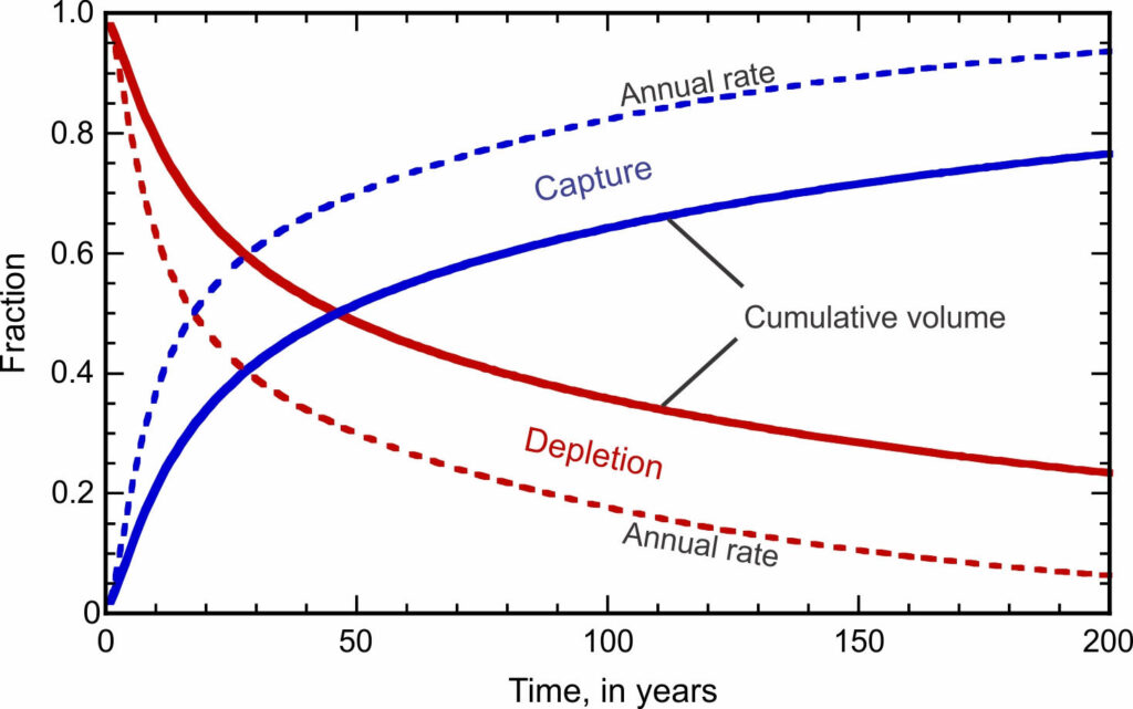
The components of the water budget changed substantially during the 200-year transient simulation period (Figure 21). After the pumping begins, well discharge is initially balanced completely by groundwater storage depletion. However, over time, more and more well discharge becomes balanced by capture and less and less by storage depletion. After about 17.5 years of pumping, the amount of capture exceeds the amount of storage depletion. After 200 years, only 6.3 percent of pumping is being balanced by groundwater storage depletion while 93.7 percent of well pumping is being balanced by capture. In this case, capture is made up entirely of streamflow depletion. Streamflow depletion is composed of both induced infiltration in the upstream reaches of the river and reduced groundwater discharge to the river in its downstream reaches. As seen in Figure 21, the quantity of induced infiltration is always somewhat greater than the reduction in groundwater discharge in this particular aquifer system. The relative contributions in any particular system will always depend on the hydraulic properties and boundary conditions governing that system.

The changes in the water budget and in the sources of water balancing the pumping can also be viewed in a nondimensional way (Figure 22). These fractions can be based on either annual rates or on cumulative volumes. As with the flow rates shown in Figure 21, the fractional sources based on annual rates cross at about 17.5 years, after which capture provides most of the water being pumped by the well. However, when viewed from the perspective of cumulative volumes of water pumped, the crossover does not occur until much later in time – at about 46 years after pumping started.
Low ET Case (Phreatophytes)
To illustrate the effects of evapotranspiration (ET) on the flow system, the base case was modified by allowing the ET process to be represented in the simulation model. The extinction depth was set to 6.0 m, and the maximum ET rate was limited to a relatively low rate of 1.72×10⁻⁵ m/d (6.28 mm/yr), yielding a linear change in ET between the extinction depth and a water table depth at the land surface (Figure 23).
The steady-state predevelopment scenario was simulated first with the addition of ET, followed by 200 years of pumping identical to the pumping rate in the base case. The calculated water budget for this case (Table 3) shows that the relatively low ET rate per unit area becomes a substantial stress for the aquifer when spread out over the large extent of the aquifer (about four times that of the pumping stress). This presence of ET in the predevelopment model results in groundwater loss and therefore lowers the groundwater level. This additional ET stress under predevelopment conditions (8,163 m3/d) lowers heads enough to induce almost twice the infiltration from the river into the aquifer (compare 5,785 m3/day in Table 1 to 9,702 m3/day in Table 3). The lower heads also cause a 57 percent reduction in groundwater discharge back out to the river in the downstream reaches of the river (compare 7,473 m3/d in Table 1 to 3,231 m3/d in Table 3). The actual ET rate varies spatially because the depth to the water table varies, and over the area of the aquifer averages 1.5 mm/yr. Because of this additional ET consumptive loss relative to the base case, under predevelopment conditions the streamflow out of the last river reach is reduced to 13,530 m3/d (compared to 21,688 m3/d in the base case with no ET). That is, the ET loss from the aquifer is completely balanced by a reduction in streamflow out of the study area.
Table 3 – Groundwater budgets for model case with low ET rate for predevelopment conditions and after 200 years of pumping one well. All flux values are in m3/d.
| Predevelopment | t = 200 Years | ||
| IN | Mountain Front Recharge | 1,688 | 1,688 |
| Change in Storage | 0 | 63 | |
| Stream infiltration | 9,702 | 11,199 | |
| Total | 11,390 | 12,950 | |
| OUT | Wells | 0 | 2,026 |
| Evapotranspiration | 8,163 | 7,844 | |
| Discharge to Stream | 3,231 | 3,084 | |
| Total | 11,394 | 12,954 |
During the 200-year pumping period, the water table declines somewhat, and the depth-dependent ET loss is reduced by just 4 percent (relative to predevelopment rates). This represents captured ET, which helps offset (or balance) the pumping (Figure 24). Compared to the base case with no ET losses, after 200 years of pumping the induced infiltration rate into the aquifer is almost twice as high, and the groundwater discharge rate to the river is almost half as much as in the base case. Streamflow depletion is smaller than in the base case and total capture now includes a component of salvaged ET. Because total capture has increased, the groundwater storage depletion has decreased relative to the base case. The net effect on streamflow is that after 200 years, the streamflow out of the downstream end of the river is reduced from a predevelopment value of 13,530 m3/d to 11,885 m3/d (compared to a reduction from 21,688 m3/d to 19,790 m3/d in the base case).

ET and Recharge Case (Phreatophytes and Rainfall)
The final scenario modeled applied a diffuse recharge rate at a uniform average long-term rate of 9.0×10⁻⁵ m/d (32.8 mm/yr) to represent recharge from precipitation and irrigation. The maximum ET rate was increased from the previous scenario to 2.8×10⁻⁴ m/d (103 mm/yr); the extinction depth was kept at 6.0 m. The calculated water budget for the simulation results in this case (Table 4) shows that the ET and diffuse recharge are now the dominant components of the water budget for both predevelopment conditions and the transient pumping conditions. However, considering all diffuse surface fluxes together, the difference between the total diffuse recharge and the total ET is much smaller – a net discharge by ET flux of just 8,157 m3/d, which is not very different from the ET flux in the previous case and represents about four times that of the pumping stress.
Table 4 – Groundwater budgets for predevelopment conditions and after 200 years of pumping for case with both diffuse recharge and ET. All flux values are in m3/d.
| Predevelopment | t = 200 Years | ||
| IN | Mountain Front Recharge | 1,688 | 1,688 |
| Diffuse Recharge | 186,479 | 186,479 | |
| Change in Storage | 0 | 0 | |
| Stream infiltration | 7,439 | 8,089 | |
| Total | 195,606 | 195,256 | |
| OUT | Wells | 0 | 2,026 |
| Evapotranspiration | 194,636 | 193,260 | |
| Discharge to Stream | 975 | 974 | |
| Total | 195,611 | 196,260 |
This volumetric rate averaged over the surface area of the aquifer is equivalent to 1.5 mm/yr. But it does vary spatially (Figure 25). Because diffuse recharge is applied uniformly over the area of the aquifer, whereas ET varies as a function of depth to the water table, the net surface flux is greatest where the depth to water is the greatest and ET is the lowest, such as the western edge of the aquifer furthest from the river (Figure 25a). The net surface flux is the most negative (ET loss greater than recharge) closer to the river, where the depth to water is minimal and ET is highest. Note that the north-south banding shown in Figure 25a derives from the stepped terraces of the land surface topography (Figure 18). Contours of change in surface flux after 200 years (Figure 25b) show that the change in ET is small, except very close to the pumping well where depth to the water table increases the most after pumping starts; of course, the contours in Figure 25b parallel the drawdown around the well.

The large fluxes of recharge and ET combined with the nonuniformity of the ET, visibly affect the head distribution in the stream-aquifer system (Figure 25). Comparing Figure 25 with Figure 20b, it is evident that heads near the western edge of the aquifer are generally higher than in the base case (no recharge or ET) because recharge generally exceeds ET in most of that band, whereas heads near the eastern edge (close to the river) are generally lower in Figure 26 because ET exceeds recharge in that band. This also induces infiltration along a greater length of the river in the ET/Recharge case than in the base case, as reflected by the angle that the head contours intersect the river. The predevelopment stream infiltration into the aquifer is almost 30 percent greater than in the base case, though smaller than in the previous low-ET case. The predevelopment aquifer discharge to the stream is much smaller than in base case, as reflected by the angle that the head contours intersect the river. The predevelopment stream infiltration into the aquifer is almost 30 percent greater than in the base case, though smaller than in the previous low-ET case. The predevelopment aquifer discharge to the stream is much smaller than in the base case, and also smaller than in the previous low-ET case, in large part because the head distribution only allows groundwater discharge to the river along a short downstream reach of the river.

After 200 years of pumping, the rate of change in storage is zero. This indicates that the system has reached a new equilibrium state by this time, and as seen in Figure 27, the new equilibrium was attained after about 75 years of pumping. In contrast, a new equilibrium had not been reached in 200 years with identical pumping for both the base case and the low-ET case. The primary reason for the change in relations here is that the much higher absolute magnitude of ET in this case permits much more of this ET discharge to be captured (or salvaged) to offset (or balance) the pumping, and it can happen faster than streamflow depletion. It is faster because streamflow capture requires time for the drawdown effects to propagate to the stream boundary, whereas ET capture occurs immediately and locally as the water table declines. Furthermore, recharge in this model scenario is a specified flux condition, and it is not affected by pumping or by drawdown. Because ET salvage is so fast and so large, the impact of pumping on streamflow is much less than in either previous case. Similarly, less groundwater storage depletion is needed to balance pumping. When storage depletion reaches zero, it means that heads have stabilized and no additional drawdown is occurring. This is the very definition of an equilibrium condition in an aquifer.

After 200 years of pumping, the stream infiltration into the aquifer has decreased by 9 percent, but the groundwater discharge to the river has stayed at about the same low rate. The streamflow leaving the downstream end of the river is 13,536 m3/d during predevelopment conditions, and that is reduced to 12,884 m3/d after 200 years of pumping. This decrease in streamflow of about 652 m3/d over time is less than half that in the low-ET case, and the fractional (nondimensional) proportion of pumping balanced by streamflow depletion is smaller than in the low-ET case (compare Figure 27 with Figure 24). Again, this is because a much greater fraction of pumping is more readily balanced by salvage (or capture) of ET losses from the aquifer.
Running the Model
The procedure for obtaining the model files, running the three scenarios presented for Case Study 1, post-processing the model outputs, and viewing the model results are explained in Box 3. The post-processing includes: creating contour maps of head and drawdown, plots of the water budget through time, calculating changes in streamflow with time, and plotting well hydrographs (i.e., water level as a function of time in a well).
Summary
Idealized hypothetical aquifers can be simulated to illustrate cause and effect relations in stream-aquifer systems. The simulations presented here have shown that groundwater withdrawn by wells must be balanced by a combination of increased recharge, decreased discharge, and depletion of groundwater in storage in the aquifer. An archive of the models, including input and output files, used to simulate the three primary scenarios described in this section are available in the file “CaseStudy1–Models.zip” as part of the online Supplemental Materials for this book. ET losses from the water table constitute one form of groundwater discharge, and lowering the water table can reduce ET losses. The reduction in ET can be viewed as salvaged ET, which helps balance pumping from wells. This might have environmental implications because of impacts on surface vegetation and changes in climatic conditions in areas where the evapotranspired water was contributing to precipitation. Additional changes in the fluxes between the aquifer and the bounding river also help to balance pumping, but constitute streamflow depletion. This might have environmental and legal implications because of impacts on aquatic ecosystems and existing surface water rights.
Salvaged ET can be a large component of capture. A small decrease in the ET rate over a large area can yield a large volume of water. Most salvaged ET offsets and reduces streamflow depletion. In a field setting, confirmation of ET salvage may be very difficult.
If the flow in the river were small enough that the effects of pumping caused reaches of the river to go dry, then pumping would have to be balanced by more storage depletion. The rate of head decline would be larger and the system could not reach a new equilibrium if there were no additional sources of capture.