6.2 Case Study 2: Paradise Valley, Nevada
Unlike hypothetical examples, real-world groundwater systems are complex and heterogeneous, and there are never enough data available to define their properties and boundary conditions uniquely, accurately, and precisely. Hence, analyses of such systems are always made in light and consideration of this uncertainty. Any model developed for field aquifer systems is always an approximation and always subject to improvement as additional data become available. But hydrogeologists are typically tasked with analyzing field systems — that is our job and that is our challenge — and the complexity and uncertainty do not preclude us from developing reliable and useful models for the task at hand. Therefore, we next provide an illustrative example of an analysis of an aquifer system that has been developed in historical times.
Description of Study Area
Paradise Valley, located in north-central Nevada, USA, is a typical valley in the Basin and Range topographic province of Nevada and western Utah in the western United States (Figure 28). It is a north-south trending valley, approximately 40 miles long by 10 miles wide (64 km by 16 km), extending north from the valley of the Humboldt River. The town of Winnemucca is situated along the Humboldt River to the southwest of Paradise Valley. Paradise Valley is surrounded by mountains to the east, north, and west, and open to the valley of the Humboldt River to the south.

The region is arid. A 100-year rainfall record in Paradise Valley indicates that the average precipitation is approximately 8 inches per year (200 mm/yr) (Prudic and Herman, 1996). Direct recharge from precipitation on the valley floor is assumed to be negligible. Two streams enter the valley from the northeast: Martin Creek and the Little Humboldt River. Martin Creek has been continuously monitored since the early 1920s (Figure 29). The locations of these two streams are shown in Figure 30.
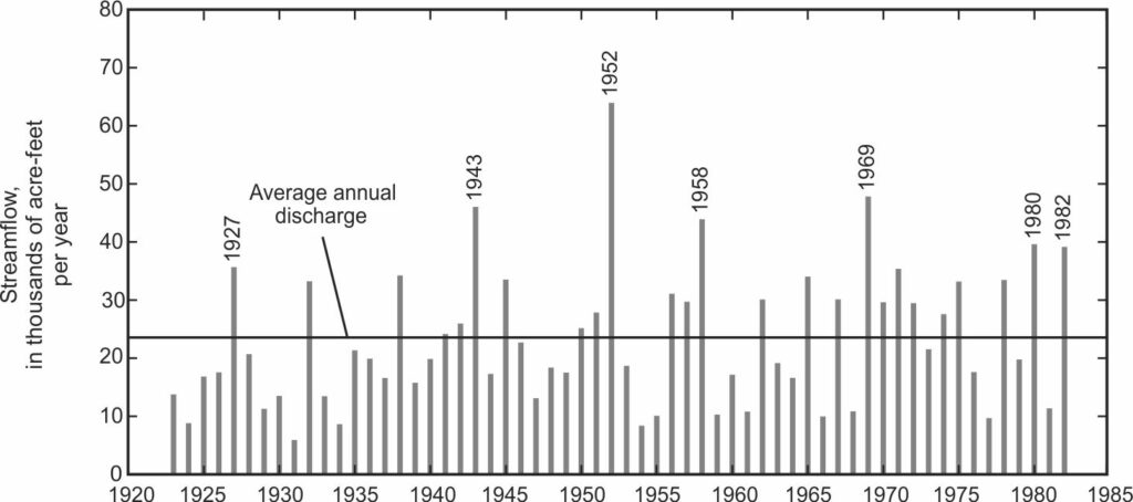
The annual discharge of Martin Creek is typical of a desert stream with wet and dry years. The Little Humboldt River is a similar stream; it has a small reservoir in the mountains to the east of Paradise Valley. There are only occasional measurements of the flow of the Little Humboldt River during the period shown on Figure 29, 1923 to 1982. With rare exceptions, all of the water from both Martin Creek and the Little Humboldt River infiltrates and recharges the alluvial aquifer in Paradise Valley near the northern end of the valley.
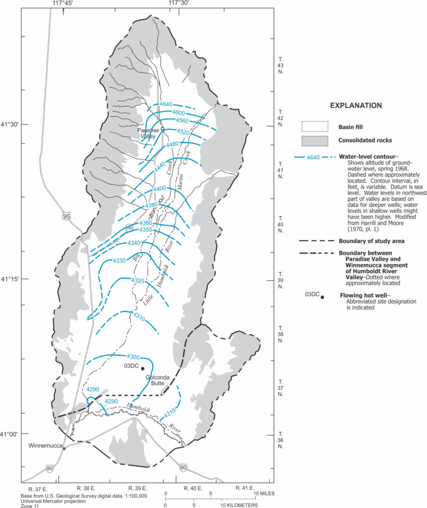
Western Nevada had a much wetter climate during the periods of Pleistocene ice advances. Lake Lahontan occupied much of western Nevada during the advance. Paradise Valley was on the fringe of the lake; two maximum rises of the lake extended into the lower reach of Paradise Valley. During the glacial period there was a through-going stream in Paradise Valley. This stream created a highly permeable alluvial deposit down the center of the valley (Bredehoeft, 1963). Paradise Valley is filled with alluvial sediments to a depth of 2,000 to 3,000 feet (600 to 900 m), but the thickness may exceed 8,000 feet (2,400 m) in the center of the valley (Prudic and Herman, 1996). The alluvium is underlain by igneous, metamorphic, and sedimentary consolidated rocks generally having low porosity and low permeability. The valley bottom slopes gently from north to south toward the Humboldt Valley. The water table generally mimics the topography of the valley floor (Figure 30).
The depth to water map (Figure 31) indicates a large area in the center of the valley where the water table is less than 10 feet (3 m) below the land surface. This is an area where phreatophytes flourished prior to groundwater development.

A reconnaissance investigation of Paradise Valley prior to significant development indicated a valley with alluvium near fully saturated with groundwater (Loeltz et al., 1949). Water from Martin Creek and the Little Humboldt River infiltrates into the alluvial aquifer within a short reach of entering the valley, as usually do the flows in all other smaller tributaries draining off the adjacent mountains. The reconnaissance studies (e.g., Loeltz et al., 1949) suggested that the average annual recharge available from the two streams, Martin Creek and the Little Humboldt River, was nearly 40,000 ac-ft/yr (0.05 km3/yr or 1.6 m3/s), which was balanced by discharge through evapotranspiration from a shallow water table over much of the valley. As shown in Figure 31, the depth to the water table is less than 30 ft (9.1 m) throughout the large central part of the valley. Groundwater discharges as evapotranspiration; much of the discharge is transpiration by phreatophytes. The thick, permeable, alluvial aquifer makes the area ideal for groundwater development. Groundwater pumping in the area increased gradually during the 1950s and 1960s, but accelerated markedly during the 1970s when it was discovered that Paradise Valley was a good place for groundwater development (Figure 32).

When irrigating, some of the water applied to a field is not used by the crop; rather, it infiltrates into the soil as groundwater recharge from irrigation. This is especially true where the water table is close to the land surface. The net pumping is the amount of pumping used by the plants or evaporated — the net pumping is the consumptive use.
Groundwater is used as the principal source for irrigation in the Paradise Valley area, and wells generally irrigate fields located close to the wells. Most of the irrigation wells in the area were drilled after 1969 and are located in the southern part of Paradise Valley (Figure 33). As the pumpage increased rapidly between 1969 and 1981, a substantial cone of depression developed in the area of heaviest pumping and irrigation in the southern part of the valley (Figure 34). Water-table declines exceeded 80 ft (24 m) in the center of the affected area. There was a decline of more than 10 ft (3 m) over a large area in the lower part of Paradise Valley.

As groundwater development increased during the 1960s and 1970s, there were management concerns about what happens to groundwater in the valley with continued pumping. Is the pumping sustainable? Would drawdown from pumping lower the water table and capture much of the evapotranspiration — leading to development that might be sustained for a long period? But a quantitative basis for assessing these questions was lacking. One approach to analyzing this question is to develop and calibrate a numerical model of the groundwater system, and then use the model to simulate the impact of continued development. In an effort to better understand the system, the USGS undertook a comprehensive numerical groundwater model study, described by Prudic and Herman (1996).

Paradise Valley Simulation Model
A three-dimensional finite-difference model was developed for Paradise Valley using the generic MODFLOW-88 model (McDonald and Harbaugh, 1988). It was conceptualized to represent varying saturated thickness, heterogeneous hydraulic properties, recharge from stream leakage, inflow from adjacent bedrock, discharge from evapotranspiration, and withdrawal by pumping wells (Figure 35). The grid used three layers, 33 columns, and 89 rows of cells. Layer thicknesses were 600 to 1,200 ft (183-366 m). Horizontal grid dimensions were 2,500 ft (762 m) on a side, and the center of each cell is designated as a node. The Humboldt River was used to simulate the southern boundary of flow in Paradise Valley, and it was simulated as a head-dependent flux boundary condition. All other boundaries were represented as no-flow boundaries, although specified fluxes are applied to some bounding cells to represent inflow from adjacent bedrock (Prudic and Herman, 1996, for details).

An Initial Steady State
The usual procedure in modeling a groundwater system is to first model the system prior to development — its undisturbed state. This procedure provides the best estimates of natural inflow (recharge) to and outflow (discharge) from the system. One uses the model to fit the observed undisturbed head distribution (Figures 30 and 31) and observed fluxes (if known). In calibrating the model, one adjusts the inflows and outflows, including their distribution, and the hydraulic parameters (such as hydraulic conductivity of the aquifer) until an adequate (or best) fit is achieved. Prudic and Herman (1996) developed a steady-state model to represent likely average conditions at the start of their transient simulations (1948).
Once one has adequately modeled the initial state of the system, the model yields a calculated water budget representative of the undisturbed system. Consistent with Equation 2, the total inflows (recharge) and outflows (discharge) under steady-state conditions are balanced (at a rate of about 74,000 ac-ft/yr [2.89 m3/s]). The Paradise Valley groundwater system is thought to be very nearly undisturbed prior to 1948 and only slightly developed during 1948-1969.
Transient Historical Simulation
Transient flow simulations were made for 1948-1982 to match the historical period of record and help assess the reliability of the model. Although the model results show substantial annual variability, Prudic and Herman (1996) report that about 60 percent of the net pumpage was derived from a reduction in storage. Therefore, about 40 percent is balanced by capture, consisting of reduced evapotranspiration, increased recharge from streams, and decreased discharge to streams.
Simulated Future Development
It was considered that future development could potentially include a prolonged total pumpage equal to about 72,000 ac-ft/yr (2.82 m3/s), an amount close to the long-term average annual streamflow into Paradise Valley. To help clarify the consequences of doing this, Prudic and Herman (1996) simulated the system under this scenario (among others) for a 300-year period of pumping. Figure 36 shows how critical inputs and outputs respond to the long 300-year period of pumping under the stresses of this proposed but hypothetical scenario.

These results indicate that not all of the phreatophyte use is captured even after 300 years of pumping; about 14,000 ac-ft/yr (0.55 m3/s) of use remains. After 300 years, pumping has induced an increase of approximately 12,400 ac-ft/yr (0.47 m3/s) in the net underflow between the Humboldt River Valley and the Paradise Valley groundwater system (by increasing underflow into Paradise Valley from the Humboldt River Valley by 10,700 ac-ft/yr and decreasing underflow out of Paradise Valley into the Humboldt River Valley by 1,700 ac-ft/yr). There is still approximately 2,600 ac-ft/yr (0.10 m3/s) continuing to be removed from storage. This means that after 300 years of pumping, the system still has not quite reached a new equilibrium state.
The drawdown after 300 years resulting from the pumping associated with this scenario exceeded 100 ft (30 m) in a large central part of the valley (Figure 37). In this particular pumping scenario, the pumping was distributed throughout the valley in the areas in which the phreatophytes grew. Drawdown in the area of riparian vegetation maximizes the capture of evapotranspiration by the pumping.
The Lesson of the Paradise Valley Example
Paradise Valley is ideally suited to groundwater development. The valley is filled with an alluvial aquifer that is both highly permeable and more than 2,000 feet (610 m) thick in most of the valley. One can drill highly productive wells in the valley. The climate, although arid, is well-suited for irrigated agriculture.
The model analysis indicates that the groundwater system in Paradise Valley was in a state of long-term equilibrium prior to development of its groundwater resources, with approximately 70,000 ac-ft/yr (2.7 m3/s) of recharge and discharge and shallow groundwater levels throughout. The principal recharge was infiltration of water from both Martin Creek and the Little Humboldt River, and the principal discharge was by riparian phreatophytes.
In creating a groundwater development system that could be maintained for a long period in Paradise Valley, the strategy was to install a pumping system that would lower the water table the most in the area of the phreatophytes and “capture” their discharge. Various alternative pumping arrangements are feasible. The scenario shown in figure 37 spreads the pumping widely up and down the valley and minimizes the drawdown for that magnitude of pumping.

In the example presented, a simulated pumping period of 300 years does not quite produce a new steady-state (equilibrium) condition. At 300 years there is still approximately 3 percent of water being removed from the system coming out of storage. This hypothetical pumping in Paradise Valley also induces a net loss of approximately 12,400 ac-ft/yr (0.48 m3/s) from the alluvial aquifer of the adjacent Humboldt River Valley. This is likely to be problematic because the additional loss of groundwater from the Humboldt River Valley alluvium will likely affect the flow of the Humboldt River, which is already fully appropriated. This is supported by observed trends in streamflow changes in the Humboldt River between the gage upstream of Paradise Valley (at Comus, Nevada, USA) and the next one downstream from Paradise Valley (near Imlay, Nevada, USA). During 1946-1975, this reach of the river consistently gained an average of 31 ft3/s (0.88 m3/s) in September, a month characterized by base flow dominance, but during 1987-2013, when groundwater pumping was substantially larger in Paradise Valley and nearby areas, the average September change in flow had been reduced to zero and the predevelopment gains in flow had been lost (D. Prudic, written communication., 2018 based on data from the USGS National Water Information System).
Even with these changes and consequences, from a hydraulic perspective the pumping scenario depicted in Figures 36 and 37 can be maintained indefinitely, as long as external factors (including climate change) do not change the average flows and capture potential from incoming and adjacent streams and additional pumping wells are not developed in the valley.