2.5 Delayed Compaction of Aquitards (Confining Beds)

An aquitard (or confining bed) is a clayey‑silty low permeability formation that does not provide an appreciable quantity of groundwater to pumping wells; however, it can transmit appreciable water to adjacent aquifers. While flow in an aquifer is predominantly two‑dimensional (2‑D) and horizontal, particularly if wellbores are fully penetrating, flow in the aquitards separating the aquifers is mostly 1‑D and vertical. In a complex aquifer system (for example, Figure 16) the role played by the intervening aquitards is important as they can represent a significant source of water to the aquifers and can contribute greatly to land subsidence as clay/silt compressibility c_b is usually much larger than that of the sand/gravel.

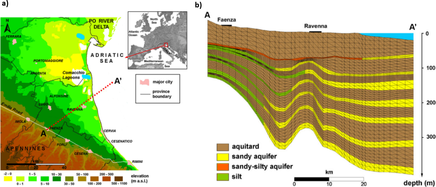
Figure 16 ‑ a) Digital elevation model of the Emilia‑Romagna plain, Italy, and b) vertical cross section along the A‑A’ alignment shown in (a) of the complex multi‑aquifer system used to supply freshwater to the coastland (modified after Teatini et al., 2006).

Normally aquitard compaction is larger and delayed in time relative to aquifer compaction. The law that governs pore-water decline in the aquitard as a function of time and the factors controlling compaction are explained in this section. Darcy’s law describing the velocity of groundwater flow in an aquitard can be written as shown in Equation 14.

(14)

where:

vz	=	apparent seepage velocity (LT-1)
K	=	hydraulic conductivity (LT-1)
h	=	hydraulic head = z + p/γ (L)
z	=	vertical coordinate positive downward (L)
∂h/∂z	=	vertical hydraulic gradient (LL-1)

The hydraulic conductivity is a function of the physical properties of fluid and soil as shown in Equation 15.

(15)

where:

k*	=	intrinsic permeability (L2)
γ	=	specific weight of water (ML-2T-2)
μ	=	dynamic viscosity of water (ML-1T-1)

Intrinsic permeability is dependent exclusively on the properties of the medium:

k* = CD²

where:

D	=	a representative length of the porous medium (for example, the average grain size) (L)
C	=	appropriate parameter related to the soil type (dimensionless)

Other more complex relationships (depending on porosity, mean pore diameter, and specific surface area) have been developed for intrinsic permeability of reactive clays, especially if salt is dissolved into the pore water (for example, Raffensperger and Ferrell Jr., 1991).

Assume the initial conditions are in equilibrium, and all the hydrologic and geomechanical quantities presented here are incremental with respect to the initial conditions. Let’s balance the weight of water in an elementary soil sample of initial length Δz and unitary cross‑sectional area (shown as 1 in the expressions below) between time t and t + Δt:

• Inflow: (γv_z) (1) (Δt)
• Outflow: γ(v_z + ∂v_z/∂z Δz) (1) (Δt)
• Weight of water expelled by the porous space contraction and the expansion of the water expressed by Equation 16 (we assume incompressible solid grains the total medium volume change coincides with the porous volume change):

−[(γ∆(ϕ∆z) 1 ∆p) + (γϕβ 1 ∆p)]

(16)

where:

β

=

volumetric compressibility of water (ML-1T-2)

In Equation 16 the total geostatic stress σ_c is assumed to be constant, so (from Equation 3):

Δσ_z = −∆p

The change in pressure, Δp, is negative when p is reduced, as happens during groundwater pumping. Notice that Δ(ϕΔz) is equal to ∆{[e/(1 + e)]∆z} with ∆z/(1 + e) constant because this is the solid part (grains) of the elementary volume (1) ∆z . Hence (from Equation 5) we have:

and therefore, we obtain:

• Outflow – Inflow = Weight of water expelled, i.e.

Cancelling γ and ∆z on both sides and remembering that the hydraulic head h = z + p/γ, we know that ∆p = γ∆h, and using Equation 14 when the increment of time approaches zero ∆t → 0 we obtain Equation 17:

(17)

Solving Equation 17, complemented with the appropriate top and bottom boundary conditions and initial conditions, provides the pressure dissipation within the aquitard, and hence the Δp needed to compute the aquitard compaction versus time. The specific storage coefficient is defined in Equation 18.

Ss = γ(cb + ϕβ)

(18)

S_s represents the “specific elastic storage” [L^‑1] and along with the hydraulic conductivity, K, defines Terzaghi’s consolidation coefficient c_v that controls both magnitude and timing of aquitard compaction as shown in Equation 19 given that ϕβ << c_b for typical aquifer confining beds.

(19)

The initial conditions correspond to Δp = 0 for the entire thickness, b, of the aquitard while the boundary conditions are given by Δp in the overlying and underlying aquifers. If the pressure drop Δp₀ is the same at top (z = 0) and bottom (z = b), then pressure conditions are symmetrical above and below the middle of the aquitard, hence ∂p/∂z = 0 at z = b/2. In this case, the solution to Equation 17 can be expressed in terms of a series expansion. Writing the solution in terms of p produces Equation 20.

(20)

where:

z	=	vertical coordinate positive downward starting from the aquitard top (0 ≤ z ≤ b/2) (L)
t	=	time since the initial change in pressure at the aquitard boundary (T)

For t = 0, and setting πz/b = x (0 ≤ x ≤ π/2) Equation 20 becomes Equation 21.

(21)

The content within the parentheses of Equation 21 is the Fourier series development of the function f (x):

Keeping in mind the range of variability of x (0 ≤ x ≤ π/2) we conclude that Equation 20 accurately represents the initial pore pressure at time t = 0.