2.1  Effective Intergranular Stress and Soil Parameters

Giuseppe Gambolati; Pietro Teatini

2.1 Effective Intergranular Stress and Soil Parameters

The theories of land subsidence are founded on basic principles of soil mechanics. Thus, the following discussion describes soil parameters, however, references to soil can be viewed as aquifer and confining bed material in a groundwater system.

The soil is viewed as a set of grains in contact. Assume a degree of saturation equal to 1 (that is, full saturation). Make a (macroscopically) horizontal cross section through the soil intersecting the contact points (Figure 11).

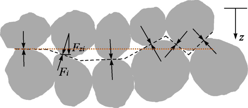
A schematic vertical cross‑section through a porous medium.

Figure 11 ‑ Schematic vertical cross‑section through a porous medium. The black dashed line is the crossing surface and the dotted orange line is the horizontal projection of the crossing surface.

Consider a piece of such a section with area A on a horizontal plane (dotted orange line, Figure 11) and n contact points (black arrows, Figure 11). If F_zi is the vertical component of the force that the grains exchange through the i^th contact area (Figure 11), we define “effective intergranular stress” σ_z by Equation 1.

$\displaystyle \sigma _{z}=\frac{\sum_{i=1}^{n}F_{zi}}{A}$

(1)

Equation 1 shows that effective intergranular stress is the uniform stress over the unit horizontal projection of a crossing surface with n contact points. Stress is a force per unit area and has dimensions of ML^-1T^-2, that is, the same dimensions as pressure. The effective intergranular stress is equivalent to the combined individual stresses, σ_zi = F_zi/A_i spread over the horizontal area, A, with stress taken to be positive in compression such that the force is the same. That is,

$\displaystyle \sigma _{z}A=\sum_{i=1}^{n}\sigma _{zi}A_{i}$

namely:

$\displaystyle \sigma _{z}=\frac{\sum_{i=1}^{n}\sigma _{zi}A_{i}}{A}=\frac{\sum_{i=1}^{n}F_{zi}}{A}$

Denote the geostatic stress by σ_c, that is, the weight of a soil column applied to a unit horizontal area at a given depth. The weight of a soil column is the combined weight of the solids and the fluids in the pores. In the case of full saturation, σ_c is equilibrated by σ_z and the pore pressure p as shown in Equation 2. The fluid pressure is distributed over the unit area minus the area of grain contacts as expressed in the parentheses of Equation 2.

$\displaystyle \sigma _{c}=\sigma _{z}+p\left ( 1-\sum_{i=1}^{n}A_{i}\textup{cos}\alpha _{i} \right )$

(2)

where:

σ_c	=	geostatic stress (ML^-1T^-2)
σ_z	=	effective intergranular stress (ML^-1T^-2)
p	=	pore pressure (ML^-1T^-2)
α_i	=	angle between the contact area, A_i, and the vertical
Ai	=	contact area normal to the force between grains (L²)

The contact area Σ(A_i cosα_i) is much smaller than 1 (as explained in Box 1), thus the quantity within the parentheses is essentially 1, hence, on first approximation, Equation 2 becomes Equation 3.

σ_c = σ_z + p

(3)

The geostatic load σ_c is also called “total vertical stress”. If σ_c remains constant during pumping (this is essentially the case for a pumped confined aquifer because pores do not drain), a decrease of p induces an equal increase of effective intergranular stress, σ_z, under whose effect the pumped formation compacts. Of course, this is a preliminary analysis. A more complete study should take into account second order effects such as the forces of mutual attraction among the grains and the fluid surface tension as well as the gas pressure in partially saturated soils.

To evaluate the compaction of a formation with decreased pore pressures we need to define a few dimensionless characteristic soil parameters:

the void ratio e, that is, the ratio of the pore volume to the grain volume; and,
the porosity ϕ, that is, the ratio of the pore volume to the total volume.

The following relationships hold:

e = PoreVolume/(TotalVolume ‑ PoreVolume) = ϕ/(1 ‑ ϕ)

ϕ = e/(1 + e)

A most important experimental profile is the behavior of e versus σ_z as derived from laboratory tests on soil samples from the compacting formation. Qualitatively, the behavior of e versus σ_z is shown in Figure 12. If the effective intergranular stress increases, the formation compacts and e decreases. As a first approximation, we assume the grains to be incompressible (the grains are much, much stiffer than the porous matrix, and especially so in shallow soils). This implies that the porous medium compaction is due essentially to the reduction of the pore volume, that is, the reduction of e and ϕ.

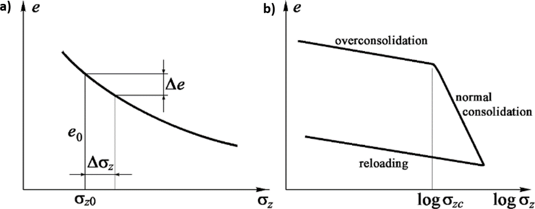
Graphs showing the typical behavior of the void ratio e against a) the effective intergranular stress σz and b) log σz.

Figure 12 ‑ Typical behavior of the void ratio e against a) the effective intergranular stress σ_z and b) log σ_z. The over‑consolidation (if present), normal consolidation, and reloading phases are highlighted on (b). Over-consolidation denotes a soil that has, in the past, experienced a maximum effective stress equal to σ_z_c that was later reduced (e.g., because of surface erosion).

The total compaction η of a layer (η has dimensions of length) as illustrated in Figure 2 (repeated here for the readers convenience) with initial thickness s₀ and initial void ratio e₀ is completely due to reduced pore space as reflected by Equation 4.

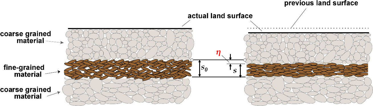
Figure showing soil compaction with a reduction of the porous space.

Repeat of Figure 2 for the reader’s convenience ‑ Soil compaction η with a reduction of the porous space (grains are incompressible for all practical purposes).

$\displaystyle \eta =s_{0}\frac{\Delta e}{1+e_{0}}$

(4)

Equation 4 is readily derived by means of the following geometric consideration: if we assume the solid grains are incompressible, the grain volume “disappeared” because of compaction must be equal to the increased volume of the grains within the compacted layer. Let A represent the horizontal area of the compacting layer. With reference to Figure 2, the grain volume loss due to compaction η is equal to ηA(1 – ϕ₀), i.e.,

ηA/(1 + e₀)

and the increased grain volume in the compacted layer is equal to sA((1 – ϕ) – (1 – ϕ₀)), that is,

$\displaystyle (s_{0}-\eta )A\left ( \frac{1}{1+e_{0}-\Delta e}-\frac{1}{1+e_{0}} \right )$

Then, equating the above two equations and rearranging yields Equation 4.

The uniaxial vertical soil compressibility c_b is the fractional change in volume, d(ΔV)/ΔV, in response to a unit change in stress, dσ_z, and has dimensions of inverse stress M⁻¹LT².

$\displaystyle c_{b}=\frac{d(\Delta V)}{dz}\frac{1}{\Delta V}$

where:

c_b	=	uniaxial vertical soil compressibility (M⁻¹LT²)
ΔV	=	volume before compaction (L³)

Since d(ΔV)/ΔV = (Pore Volume change)/(Pore Volume + Grain Volume) = Δe/(1 + e), we can substitute Δe/(1 + e) for d(ΔV)/ΔV to obtain the following expression for c_b.

$\displaystyle c_{b}=\frac{1}{d\sigma _{z}}\frac{\Delta e}{1+e}$

The uniaxial vertical soil compressibility can be expressed as shown in Equation 5 by including a minus sign so as to obtain a positive c_b value (σ_c and σ_z are assumed to be positive even though they are compressive stresses). Then, compressibility, c_b, can be estimated in the laboratory by finding the slope of the experimental profile shown in Figure 12a and evaluating Equation 5.

$\displaystyle c_{b}=\frac{de}{d\sigma _{z}}\frac{1}{1+e}$

(5)

The minus sign in the above equation is introduced so as to obtain a positive c_b value (σ_c and σ_z are assumed to be positive although they are compressive stresses). Assume c_b is constant, then Equation 5 leads to:

$\displaystyle \frac{de}{1+e}=-c_{b}d\sigma _{z}$

and integration leads to:

ln(1 + e) = −c_bσ_z + C

which simplifies to Equation 6.

$\displaystyle e=C\ \textup{exp}(-c_{b}\sigma _{z})-1$

(6)

The integration constant C is determined by prescribing that e = e₀ for σ_z = σ_z₀, thus C is:

$\displaystyle C=(1+e_{0})\textup{exp}[-(-c_{b}\sigma _{z})]$

and substituting C into Equation 6 results in Equation 7.

$\displaystyle e=(1+e_{0})\textup{exp}[-c_{b}(\sigma _{z}-\sigma _{z0})]-1$

(7)

Generally, e₀ corresponds to the initial conditions where σ_z = σ_z₀ prior to the inception of pumping. The assumption of constant c_b has validity over a limited range of σ_z. The porous medium becomes stiffer as Δσ_z increases and compaction progresses. Therefore, Equation 7 will be used for σ_z values falling within a given stress range. In general, c_b will be calculated using Equation 5 once the profile of Figure 12 is available.

License