2.2 Pumping from a Water Table Aquifer
For the sake of simplicity, assume a water table aquifer is horizontal and the piezometric decline due to pumping over a given time interval is Δz. Let θw be the moisture content (i.e., the fraction of the total porous medium volume occupied by water, moisture content is equal to porosity in a fully saturated medium) within the unsaturated zone above A, and, between the phreatic surfaces (labeled as the piezometric levels A and B in Figure 13) after the piezometric surface has declined from A to B.
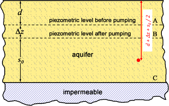
Figure 13 ‑ Sketch of a pumped water table aquifer.
As a result of lowering the piezometric level, there will be an increase of effective stress due to drainage of water from the zone between A and B because that zone is no longer under the influence of pore water pressure (Archimedes’ upward buoyant force). At any point location between B and C, the geostatic stress, σc, is decreased by the quantity γΔz(ϕ ‑ θw), with γ being the specific weight of water with dimensions ML-2T-2, and the quantity γΔz being p. Therefore, the effective stress, σz, is increased by (Equation 8),
| Δσz = γΔz(1 – ϕ +θw) | (8) |
that is to say, it is increased by the difference in Archimedes’ force exerted upon the solid grains before and after pumping. The layers underlying the water table aquifer, where p remains constant, experience a σz reduction equal to the σc reduction (that is, γΔz(ϕ ‑ θw)) with a resulting small rebound. As the magnitude of the rebound is small, it is discarded in the following calculation. Let’s refer to the mid‑point between B and C in Figure 13. The stress σz0 before withdrawal is as shown in Equation 9.
| σz0 = (1 – ϕ)[γ′(d + Δz + s0/2) − γ(Δz + s0/2)] + γθwd | (9) |
where:
| γ′ | = | specific weight of the solid grains (ML–2T-2) |
To obtain Equation 9 we used Equation 3 where σc is equal to the geostatic weight of a soil column with height h = d + Δz + s0/2, that is, σc = γθwd + γ′h(1 − ϕ) + γϕ(h − d), and p = γ(h − d). We thus locate the σz0 point in Figure 12a and, by making use of Equation 8, compute the subsidence at a given depth according to Equation 4 as follows.

It is easier to visualize the relationship between compaction and void ratio using an abstract version of Figure 2 in which all solids are grouped with no pore space and all pore space occupies the remainder of the volume, with example values assigned and calculations carried out, as explained in Box 2. Box 2 also provides a worked example of calculating the change in effective stress for a decline in the piezometric level of an unconfined aquifer as shown in Figure 13.
If s0 is large, we can divide s0 into a number of sublayers and implement the above calculation for the mid‑point of each sublayer (Δσz is the same for each sublayer while σz0 changes).
In summary, the compaction of a phreatic aquifer is shown in Equation 10.
 |
(10) |
In Equation 10, cb is the uniaxial vertical soil compressibility, and Δσz is the change in the effective intergranular stress (Equation 8).