Box 3 3‑D Poroelasticity Equations

Giuseppe Gambolati; Pietro Teatini

Box 3 3‑D Poroelasticity Equations

Theoretically, land subsidence is best analyzed according to the theory of consolidation (Biot, 1941), which holds that consolidation itself represents the response of a compressible porous medium to changes in the flow field operating within it. A complete analysis of land subsidence requires determination of the 3‑D deformation field accompanying the 3‑D flow field, and must be accomplished in a complex multi‑aquifer system. A few basic principles underlie the consolidation process. As outlined above, the first principle advanced by Terzaghi (1923) states that the total stress σ_tot at any point of the porous medium is equal to the sum of the effective intergranular σ_eff and the neutral pore pressure p:

σ_tot = σ_eff + p

Deformation of the porous body is controlled exclusively by variation of the effective stress σ_eff. If we consider changes relative to an initial undisturbed state of equilibrium, the Cauchy equations of equilibrium are cast in terms of incremental effective stress and pore pressure as shown in Equation Box 3‑1.

	$\displaystyle \frac{\partial \sigma _{xx}}{\partial x}+\frac{\partial \tau _{xy}}{\partial y}+\frac{\partial \tau _{xz}}{\partial z}=\frac{\partial p}{\partial x}$
	$\displaystyle \frac{\partial \tau _{yx}}{\partial x}+\frac{\partial \sigma _{yy}}{\partial y}+\frac{\partial \tau _{yz}}{\partial z}=\frac{\partial p}{\partial y}$	(Box 3-1)
	$\displaystyle \frac{\partial \tau _{zx}}{\partial x}+\frac{\partial \tau _{zy}}{\partial y}+\frac{\partial \sigma _{zz}}{\partial z}=\frac{\partial p}{\partial z}$

where:

σ_xx	=	incremental normal effective stress in x direction
σ_yy	=	incremental normal effective stress in y direction
σ_zz	=	incremental normal effective stress in z direction

and, the incremental shear stresses:

τ_xy	=	τ_yx
τ_xz	=	τ_zx
τ_yz	=	τ_zy

The relationships between the incremental effective stress tensor σ and the incremental strain tensor ε for a geomechanical isotropic medium are shown in Equation Box 3‑2.

$\displaystyle \begin{bmatrix} \sigma _{xx} \\ \sigma _{yy} \\ \sigma _{zz} \\ \tau _{xy} \\ \tau _{xz} \\ \tau _{yz}\end{bmatrix}=D^{-1}\begin{bmatrix} \varepsilon _{xx} \\ \varepsilon _{yy} \\ \varepsilon _{zz} \\ \varepsilon _{xy} \\ \varepsilon _{xz} \\ \varepsilon _{yz}\end{bmatrix}$

(Box 3-2)

with matrix D^-1 as shown in Equation Box 3‑3.

$\displaystyle D^{-1}=\frac{E}{(1+\nu )(1-2\nu )} \begin{bmatrix} 1-\nu & \nu & \nu & 0 & 0 & 0 \\ \nu & 1-\nu & \nu & 0 & 0 & 0 \\ \nu & \nu & 1-\nu & 0 & 0 & 0 \\ 0 & 0 & 0 & \frac{1-2\nu }{2} & 0 & 0 \\ 0 & 0 & 0 & 0 & \frac{1-2\nu }{2} & 0 \\ 0 & 0 & 0 & 0 & 0 & \frac{1-2\nu }{2} \\ \end{bmatrix}$

(Box 3-3)

where:

E	=	Young’s modulus (stiffness of a solid as the ratio of its tensile stress and axial strain, ML^-1T^-2)
ν	=	Poisson’s ratio (reflects deformation of a solid in the direction perpendicular to loading, the negative ratio of transverse strain to axial strain, dimensionless)

Typically, in layered aquifer systems laid down in a depositional environment, the geomechanical properties along the vertical direction (v) are different from those in a horizontal direction (h). The geomechanical properties of a transversally isotropic porous medium are fully described by five independent parameters E_v, E_h, v_v_, E_h, G_v, with G the shear modulus. G_h is dependent on E_h and v_h through Equation Box 3‑4.

$\displaystyle G_{h}=\frac{E_{h}}{2(1-\nu _{h})}$

(Box 3-4)

Thermodynamic consistency requires the positive definiteness of matrix C ⁻¹ relating the stress tensor to the strain tensor, which implies (Ferronato et al., 2013):

$\displaystyle 1-\nu {_{h}}^{2}>0$ and $\displaystyle 1-\nu {_{h}}-2\nu {_{h}}^{2}\frac{E_{v}}{E_{h}}>0$

then, as shown in Equations Box 3‑5, setting,

	$\displaystyle \vartheta =\frac{E_{h}}{E_{v}}$
	$\displaystyle \eta =\frac{E_{h}}{2(1+\nu _{h})G_{v}}$	(Box 3-5)
	$\displaystyle \alpha =\frac{1}{E_{v}}\left ( 1-\frac{2\nu {_{v}}^{2}}{1-\nu _{h}}\frac{E_{v}}{E_{h}} \right )$

the constitutive matrix C ^–¹ (equivalent to D^-1 for a transversally isotropic medium) is Equation Box 3‑6 (Ferronato et al., 2013).

$\displaystyle C^{-1}=\frac{1}{(1-\nu {_{h}}^{2})\alpha }\begin{bmatrix} C{_{1}}^{-1} & 0 \\ 0 & C{_{2}}^{-1} \\ \end{bmatrix}$

(Box 3-6)

where:

$\displaystyle C{_{1}}^{-1}=\begin{bmatrix} \vartheta -\nu {_{v}}^{2} & \nu {_{v}}^{2}+\vartheta \nu _{h} & \nu _{v}(1+\nu _{h}) \\ \nu {_{v}}^{2}+\vartheta \nu _{h} & \vartheta -\nu {_{v}}^{2} & \nu _{v}(1+\nu _{h}) \\ \nu _{v}(1+\nu _{h}) & \nu _{v}(1+\nu _{h}) & 1-\nu {_{v}}^{2} \\ \end{bmatrix}$

$\displaystyle C{_{2}}^{-1}=\frac{\vartheta (1-\nu _{h})-2\nu {_{v}}^{2}}{2}\begin{bmatrix} 1 & 0 & 0 \\ 0 & 1/\eta & 0 \\ 0 & 0 & 1/\eta \\ \end{bmatrix}$

The coefficient α provided in Equation Box 3‑5 is the vertical oedometric compressibility of the medium prevented from expanding laterally (Gambolati et al., 1984). Setting v_h= v_v, E_h = E_v, and G_h = G_v, Equation Box 3‑6 becomes Equation Box 3‑2 and α becomes Equation Box 3‑7.

$\displaystyle \alpha =\frac{(1+\nu )(1-2\nu )}{(1-\nu )E}$

(Box 3-7)

Equation Box 3‑7 is the vertical compressibility of an isotropic soil. If we replace the relations between the effective stress and the strain above into the Cauchy equations, we obtain the equilibrium equations for a porous medium subject to internal pore pressure variations, p, written in terms of displacements (isotropic medium) as in Equation Box 3‑8.

	$\displaystyle G\triangledown ^{2}u+(\lambda +G)\frac{\partial \varepsilon }{\partial x}=\frac{\partial p}{\partial x}$
	$\displaystyle G\triangledown ^{2}u+(\lambda +G)\frac{\partial \varepsilon }{\partial y}=\frac{\partial p}{\partial y}$	(Box 3-8)
	$\displaystyle G\triangledown ^{2}u+(\lambda +G)\frac{\partial \varepsilon }{\partial z}=\frac{\partial p}{\partial z}$

where:

u, v, w	=	components of the incremental position vector along the coordinate axes x, y, and z, respectively (L)
∇²	=	Laplace operator
λ	=	Lamè constant equal to νE/[(1 – 2ν) (1 + ν)]
ε	=	ε_xx + ε_yy + ε_zz, volume strain or dilatation

Similar equations hold for a transversally isotropic medium, not given here, however, because of their greater complexity. There are three equations with four unknowns: u, v, w, and p. The additional equation needed to close the system is provided by the groundwater flow equation that controls subsurface flow within the aquifer.

The flow equation is based on the principle of mass conservation for both solid grains and water. Thus, Darcy’s law must be cast in terms of the relative velocity of fluid to grains. Cooper (1966) and Gambolati (1973a) derived the flow equations by assuming a grain velocity different from zero, and worked with material derivatives (total derivatives and substantial derivatives) in the appropriate places in the development. Gambolati (1973b) showed that the grain velocity can be discarded, that is, assumed to be zero, as long as the final soil settlement does not exceed 5 percent of the original aquifer thickness, a condition reached in nearly all applications. DeWiest (1966) took into consideration the dependence of the hydraulic conductivity on the water’s specific weight, γ, via the intrinsic permeability and the dependence of γ on the incremental pressure variation. Gambolati (1973b) again showed that the influence of the dependence of γ on the hydraulic conductivity is slight, and can safely be neglected. Later, within this framework, the groundwater flow equation as originally developed by Biot (1941, 1955) was elegantly and clearly derived by Verruijt (1969), and thus the fourth equation to be added to the above Equation Box 3‑8 is Equation Box 3‑9.

$\displaystyle \frac{1}{\gamma }\triangledown \cdot (K_{ij}\triangledown p)=\phi \beta \frac{\partial p}{\partial t}+\frac{\partial \varepsilon }{\partial t}$

(Box 3-9)

where:

∇	=	∂/∂x + ∂/∂y + ∂/∂z
K_ij	=	k_ijγ/μ, hydraulic conductivity tensor with principal components K_xx, K_yy, and K_zz
k_ij	=	intrinsic permeability tensor
μ	=	viscosity of water
ϕ	=	medium porosity
β	=	compressibility of water

Equation Box 3‑8 together with Equation Box 3‑9 form the mathematical basis of the so‑called “coupled” (or Biot) formulation of flow and stress in an isotropic porous medium experiencing groundwater flow. It is the most sophisticated theoretical approach to the simulation of land subsidence in the area of linear elasticity. Gambolati (1974) showed that at any point P of the porous medium, the deformation may be expressed as the sum of two contributing factors: (1) the pointwise deformation caused by the incremental pore pressure acting at P and (2) the deformation caused by the pressure p acting outside P, namely in the remainder of the medium. Gambolati (1974) called the second factor the “three‑dimensional effect”: it vanishes, of course, in one‑dimensional media. The first factor is expressed as:

$\displaystyle \varepsilon =\frac{1}{E_{v}}\left ( 1-\frac{2\nu {_{v}}^{2}}{1-\nu _{h}}\frac{E_{v}}{E_{h}} \right )p=\alpha p$

in a geomechanical transversally isotropic medium, and

$\displaystyle \varepsilon =\frac{(1+\nu )(1-2\nu )}{(1-\nu )E}p=\alpha p$

in a geomechanical isotropic medium, with α the vertical compressibility previously defined. Replace the above expression for ε in the flow Equation Box 3‑9) and you obtain the so‑called “uncoupled” formulation of flow and stress. In the uncoupled formulation the flow equation is solved for p independently of the stress equation, with the gradient of the pore pressure variations later integrated into the equilibrium equations (Equation Box 3‑8) as a known external source of strength. The uncoupled flow equation is thus Equation Box 3‑10.

$\displaystyle \triangledown \cdot (K_{ij}\triangledown p)=\gamma (\alpha +\phi \beta )\frac{\partial p}{\partial t}$

(Box 3-10)

Assuming the medium to be transversally isotropic as far as the hydraulic conductivity is concerned as well, having axes coincident with the principal directions of anisotropy, Equation Box 3‑10 becomes Equation Box 3‑11.

$\displaystyle \frac{\partial }{\partial x}\left ( K_{xx}\frac{\partial p}{\partial x} \right ) +\frac{\partial }{\partial y}\left ( K_{yy}\frac{\partial p}{\partial y} \right ) +\frac{\partial }{\partial z}\left ( K_{zz}\frac{\partial p}{\partial z} \right ) =S_{s}\frac{\partial p}{\partial t}$

(Box 3-11)

The coefficient S_s= γ(α + ϕβ) is the specific elastic storage coefficient referred to previously. The uncoupled equation has been the basis of classical groundwater hydrology from the very beginning of quantitative hydrogeology’s development (for example, Theis, 1935; Jacob, 1940; Todd, 1960; and Bear, 1972), and is still universally used today. The superiority of the coupled approach in predicting land subsidence due to groundwater pumping has been disputed by Gambolati et al. (2000), who showed that the uncoupled pressure solution can be safely used in predicting land subsidence in compacting sedimentary basins, the coupled and uncoupled solutions being virtually indistinguishable at any time of practical interest.

It may also be of interest to mention some basic definitions of oedometer vertical soil compressibility, which is the main rock parameter controlling land subsidence. The definition of α given above is the one derived from the classical theory of elasticity assuming reversible elastic properties of the porous medium. The problem of defining various rock compressibilities is thoroughly discussed by Zimmerman (1991). In the present analysis, we restrict our discussion to the comparison between α as defined above, and the compressibility c_b as is typically defined in geotechnics by Equation Box 3‑4). Assume a 1‑D soil sample with initial length Δz experiencing a vertical (oedometer) deformation δ(Δz). In the classical elastic theory, the vertical compressibility α is defined as Equation Box 3‑12:

$\displaystyle \alpha =\frac{\delta (\Delta z)}{\Delta z}\frac{1}{p}=\frac{\varepsilon}{p}$

(Box 3-12)

where

p

, equal and opposite to the incremental effective stress, is negative in the sample compaction δ(Δz). Using the void ratio, we can write Equation Box 3‑13:

$\displaystyle \delta (\Delta z)=[\Delta z+\delta (\Delta z)]\frac{e}{1+e}-\Delta z\frac{e_{0}}{1+e_{0}}$

(Box 3-13)

where:

e₀

=

initial void ratio prior to compaction (Figure 2)

Equation Box 3‑13 assumes that the individual soil grains are incompressible, so that the sample volume δ(Δz) is equal to the variation of the porous volume (Figure 2). By dividing both sides of Equation Box 3‑13 by Δz and rearranging, we obtain Equation Box 3‑14.

$\displaystyle \varepsilon =\frac{\delta (\Delta z)}{\Delta z}=\frac{e-e_{0}}{1+e_{0}}$

(Box 3-14)

also,

$\displaystyle \alpha =\frac{\varepsilon }{p}=\frac{e-e_{0}}{p(1+e_{0})}$

and if α does not depend on p then Equation Box 3‑15 can be written.

$\displaystyle \frac{de}{dp}=\alpha (1+e_{0})$

(Box 3-15)

That is, the void ratio is proportional to the incremental pressure p (for any given initial e₀). Substitution of Equation Box 3‑15 into Equation 5 of the main portion of this book, with dp = −dσ_z, leads to:

$\displaystyle c_{b}=\alpha \frac{1+e_{0}}{1+e} =\alpha \frac{1+e_{0}}{1+e_{0}+\alpha p(1+e_{0})} =\frac{\alpha }{1+\alpha p}$

Only when the incremental pressure p approaches 0, do α and c_b coincide. In general, the two compressibilities α and c_bare not equal and cannot be considered simultaneously constant. The expression of c_b versus ε is (using Equation Box 3‑14) is as shown in Equation Box 3‑16.

$\displaystyle c_{b}=\frac{1+e_{0}}{1+e}\frac{d\varepsilon }{dp} =\frac{1}{1+\varepsilon }\frac{d\varepsilon }{dp}$

(Box 3-16)

If α is constant and dε/dp = α we have Equation Box 3‑17.

$\displaystyle c_{b}=\frac{\alpha }{1+\varepsilon }=\frac{\alpha }{1+\alpha p}$

(Box 3-17)

Gambolati (1973b) has shown that the assumption of constant α can be easily removed to give the general correct relationship between α and c_b as in Equation Box 3‑18.

$\displaystyle c_{b}=\frac{p\frac{d\alpha }{dp}+\alpha }{1+\alpha p }$

(Box 3-18)

If c_b is constant, Equation Box 3‑18 can be integrated to provide α as expressed in Equation Box 3‑19.

$\displaystyle \alpha =\frac{\textup{exp}(pc_{b})-1}{p}$

(Box 3-19)

The assumption that the individual grains are incompressible is fully warranted by the fact that the compressibility of any aquifer system is orders‑of‑magnitude greater than the compressibility of the single grain. Geerstma (1973) provides the value of α = 1.610^‑⁶ bar^‑¹ for grains of silicate. In contrast, the compressibility of aquifer systems is, typically, orders‑of‑magnitude larger than the compressibility of single grains as shown in Figure Box 3‑1. Figure Box 3‑1 provides an example of the compressibility of an aquifer system in terms of the relationship of α versus depth and vertical effective intergranular stress σ_z_z in the sedimentary basin of the river Po plain, Italy (Gambolati et al., 1991, 1999; and Comerlati et al., 2004). However, as long as the ultimate relative compaction αp does not exceed 5 percent of the compacting unit (which is typically the case in geologic formations, particularly in shallow formations), the difference between α and c_b does not exceed 2‑3 percent (Gambolati, 1973b, Figure 14) and for practical applications the two definitions are interchangeable.

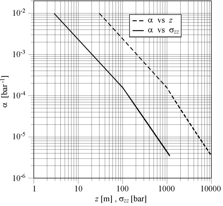
Graph of uniaxial vertical compressibility versus effective stress and depth in the Po river plain, Italy.

Figure Box 3‑1 ‑ Uniaxial vertical compressibility, α, versus effective stress σ_zz and depth z in the Po river plain, Italy (after Comerlati et al., 2004).

Finally, it is worth mentioning that, when comprehensive in situ and lab soil characterizations are available, more realistic constitutive formulations taking into account plastic or viscoplastic behavior may be developed and used for the simulation and prediction of land subsidence in soft under‑consolidated alluvial basins (for example, Ye et al., 2012).

Return to where text linked to Box 3

License