2.6  Time Factor and Compaction Profile

Giuseppe Gambolati; Pietro Teatini

2.6 Time Factor and Compaction Profile

The (positive) compaction η(t) of the half aquitard at time t is:

$\displaystyle \eta (t)=\int_{0}^{b/2}c_{b}(p_{0}-p)dz$

Substituting Equation 20, and integrating term by term leads to Equation 22.

$\displaystyle \eta (t)=\frac{4}{\pi ^{2}}c_{b}\Delta p_{0}b\sum_{n=0}^{\infty }\frac{1}{(2n+1)^{2}}\left\{1-\frac{1}{\textup{exp}\left ( [(2n+1)\pi /b]^{2}c_{v}t \right )} \right\}$

(22)

For t = 0 we get η(0) = 0, while for t = ∞ Equation 22 becomes Equation 23.

$\displaystyle \eta (\infty )=\frac{4}{\pi ^{2}}c_{b}\Delta p_{0}b\left ( 1+\frac{1}{3^{2}}+\frac{1}{5^{2}}+\frac{1}{7^{2}}+... \right )$

(23)

The above series converges to π²/8 and therefore η(∞) is the ultimate compaction of the half aquitard, as was already pointed out for the various aquifers represented by Equations 4 and 5 and is expressed here as Equation 24.

$\displaystyle \eta (\infty )=c_{b}\Delta p_{0}\frac{b}{2}$

(24)

It may be interesting to compute the time needed by the aquitard to achieve a given percentage of full compaction, η(∞), provided by Equation 24. To this aim we introduce the dimensionless time factor T_v (Equation 25) as defined by Terzaghi (1923).

$\displaystyle T_{v}=4\frac{c_{v}t}{b^{2}}$

(25)

Denoting the percentage compaction as w, Equation 26 shows that it is a function of only T_v.

$\displaystyle w(T_{v})=\frac{8}{\pi ^{2}}\sum_{n=0}^{\infty }\frac{1}{(2n+1)^{2}}\left\{1-\frac{1}{\textup{exp}[\pi ^{2}(2n+1)^{2}T_{v}/4]} \right\}$

(26)

The behavior of w(T_v) is shown in Figure 17. There are basically two ways to use Figure 17:

enter Figure 17 with a given percent of the final compaction, to obtain the corresponding T_v and calculate the time t needed to reach that percentage from Equation 25; or,
select a time t, compute T_v from Equation 25 and derive the percentage compaction from Figure 17.

The compaction of the aquitard at time t is shown as Equation 27.

η(t) = 2w(T_v) η(∞) = w(T_v) c_bΔp₀b

(27)

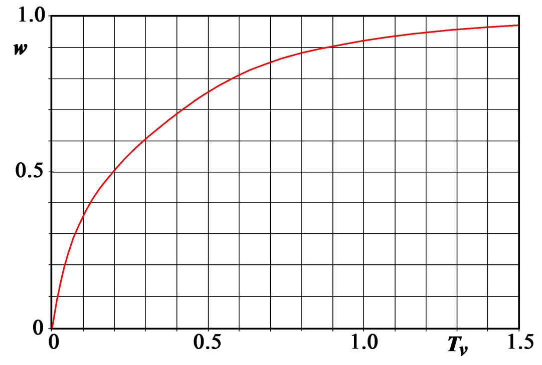
Figure 17 ‑ Behavior of the aquitard compaction η(t) relative to the ultimate compaction η(∞), c_bΔp₀b versus time factor T_v_.

Figure 17 is also helpful to compute the compaction of an aquitard that is in contact with a non‑productive aquifer, for example, with Δp₀= 0 at the aquitard bottom. In fact, notice that because of the linearity of Equation 17 and, with Δp₀ equal on both aquitard top and aquitard bottom, we can superpose the effects, namely we can separately compute the compaction of the aquitard subject to Δp₀ ≠ 0 on top and Δp₀ = 0 on bottom and vice versa Δp₀ = 0 on top and Δp₀ ≠ 0 on bottom. The Δp behavior versus z for various time values is shown in Figure 18 from right and left respectively.

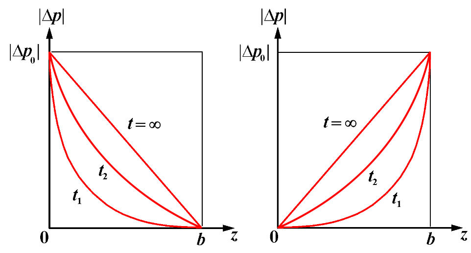
Figure 18 ‑ Schematic behavior of the pore pressure decline in an aquitard subject to an instantaneous pore pressure drop Δp₀ on top (z = 0, left) and bottom (z = b, right) for representative time values.

The area underlying a Δp₀ profile at any given time, for instance t₁_, is the same on the left and right images of Figure 18. Such an area, however, is proportional to the compaction of the aquitard subject to Δp₀ ≠ 0 on both top and bottom, that is, half the value η(t) provided by Equation 22. In summary, if one of the adjacent aquifers is not pumped the aquitard compaction is given by Equations 22 and 24 at current time t and t = ∞ respectively. We can use the graph of Figure 17 as explained earlier with the percent compaction relative to the final compaction described by Equation 24.

A straightforward generalization is the implementation of the previous outcome to the case where aquifers top and bottom experience different pore pressure drops, that is, Δp₁ ≠ Δp₂. The ultimate aquitard compaction is given by Equation 28.

$\displaystyle \eta (\infty )=\frac{1}{2}(\Delta p_{1}+\Delta p_{2})c_{b}b$

(28)

Figure 17 may be used as described above along with the percentage relative to η(∞) of Equation 26. In case for which the pore pressure drops Δp₁ and Δp₂ on top and bottom of the aquitard are a continuous function of time, they can be approximated with stepwise functions with the effects of the incremental drops superposed at the corresponding times.

License