Hydraulic gradient (Δh/ΔL) is often expressed mathematically in differential format as dh/dL. Rearrangement of Darcy’s law using this formulation shows that hydraulic gradient is a function of Q, K, and A:

(4)

Therefore, a change in any one of these variables will manifest as a change in hydraulic gradient:

(5)

(6)

(7)

The negative sign is due to the fact that water flows in a direction from higher head to lower head, as described previously. The term –dh/dL represents the slope of the head decline in the direction of flow (the “steepness” of the hydraulic gradient).

Figure 5 summarizes this concept using three different, yet spatially-uniform scenarios. The hydraulic gradient, which is commonly measured by way of water levels in wells, is not the controlling parameter that dictates flow. Rather, hydraulic gradient is a manifestation of the combined effects of the system geometry, hydrogeologic properties and the flow rate imposed on the system.

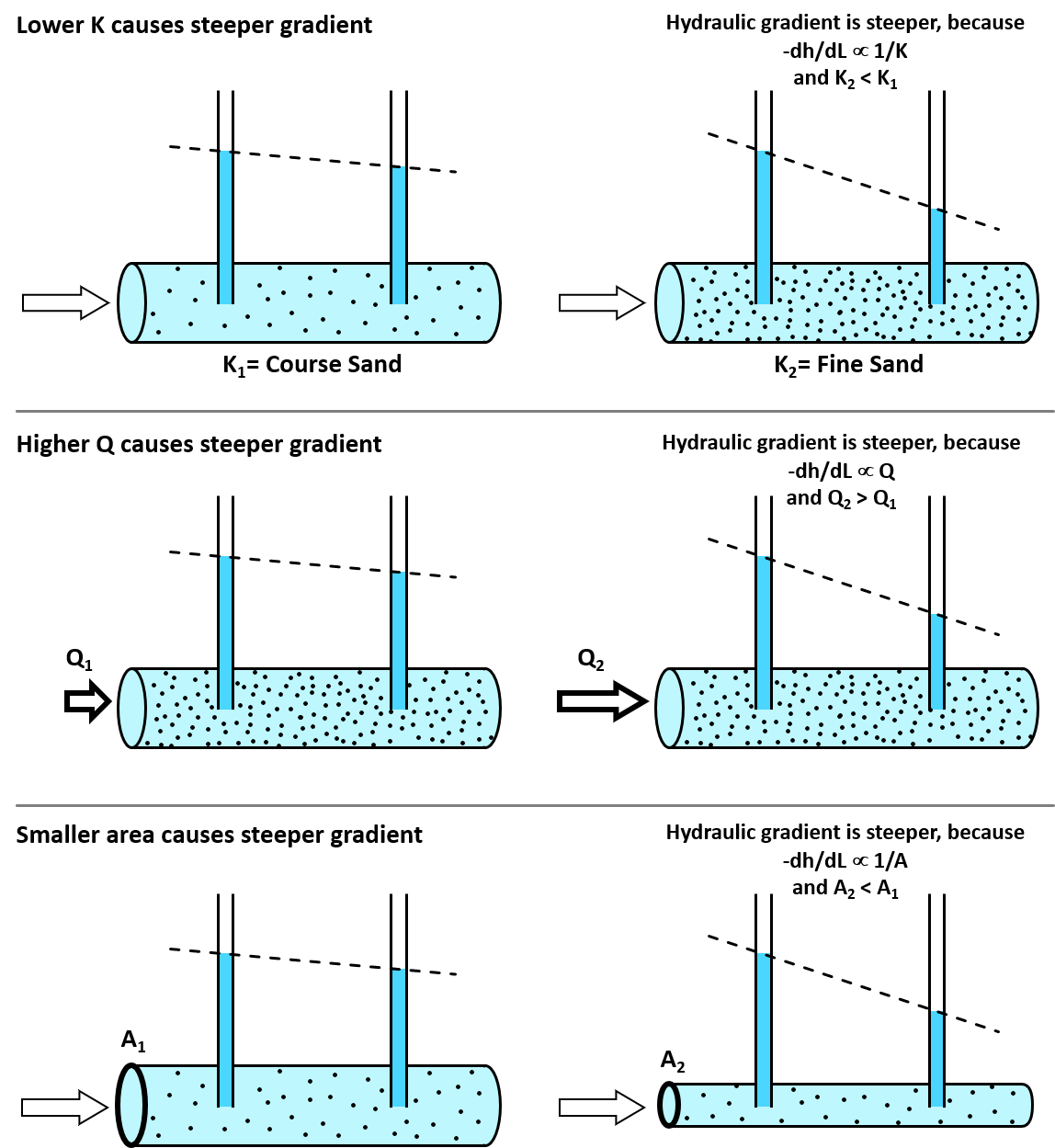
Figure 5 – Illustration of hydraulic gradient dependence on hydraulic conductivity, flow rate, and area. In each case, the gradient changes in accordance with the proportionality relationship defined by Darcy’s law (Cohen and Cherry, 2020).

In the example shown in Figure 6, K₂<K₁ whereas Q and A are constant. Q is the same at every location along the tube because mass is conserved. Therefore, as indicated by Darcy’s law, the gradient in the region of K₂ must be steeper than in the other regions. This simple scenario is an example of a heterogeneity; in this case, hydraulic conductivity is not uniform.

Figure 6 – Change in hydraulic gradient due to variable hydraulic conductivity. In this case, the gradient is steeper in the section with lower K, since gradient is inversely proportional to K (Cohen and Cherry, 2020).

Example Problem 1

Sketch the horizontal hydraulic head gradient along the length of the apparatus shown here in a manner similar to the way the gradient is shown in Figure 6 (there is no need to know the actual head values, so you can create your own relative values).

Click here for solution to Example Problem 1