3.10 Calibrating Groundwater Models

A groundwater model is a mathematical representation of a groundwater system created using estimates of hydraulic parameters and boundary conditions. Given the properties and boundaries, a solution of the model provides hydraulic heads and flow rates within the groundwater system. These simulated heads and flows are compared to the heads and flows measured in the field and, if they do not match, the properties and boundaries are adjusted to improve the match between the model output and the measured data. This adjustment process is calibration of the model. However, when both aquifer properties (e.g., K) and boundary fluxes (e.g., recharge and discharge) are unknown, the calibration process does not produce a unique estimate of properties or fluxes.

Many numerical groundwater models now offer the opportunity to simulate the distribution of groundwater ages and/or tracer concentrations within aquifer systems. When using groundwater ages to estimate aquifer recharge, numerical models allow for consideration of more realistic aquifer geometries than provided by the simple models discussed above (e.g., Figure 14). They also offer the opportunity for comparison between simulated and measured groundwater ages (or tracer concentrations), to evaluate the quality of model calibration. Use of groundwater age tracers for model calibration has the potential to overcome some of the non-uniqueness that is often involved with calibration of models using only hydraulic head data (Sanford, 2011).

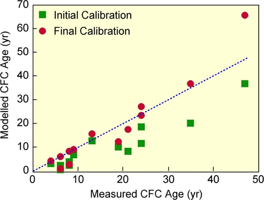
One of the earlier studies that illustrated this application of groundwater age data was published in the early-1990s, and used the United States Geological Survey software (USGS, 2019) to create a two-dimensional model of hydraulic heads and flow in the agricultural Locust Grove catchment (Section 3.9). The initial calibration of the model (that did not involve groundwater ages) used values for recharge (457 mm/y) and hydraulic conductivity (K_h = 30.5 m/d with anisotropy ratio of 5:1) based on previous studies, and these values were consistent with observed hydraulic heads. A groundwater travel time analysis was then performed using the United States Geological Survey MODPATH software (USGS, 2019) to track particles in the simulated groundwater system, assuming a porosity value of 0.3. Travel times indicated by MODPATH were much smaller than those estimated from CFC-12 measurements on observation wells within the catchment (Figure 44). This suggested that the recharge rate should have been lower; the fit to heads can be maintained by keeping recharge and hydraulic conductivity in the same ratio. The model was then recalibrated until a much better fit to the CFC-12 ages was obtained, while retaining acceptable fit to heads. The final calibrated model used an average recharge rate of 305 mm/y, and horizontal hydraulic conductivity of 16.8 m/d.

The study described above used the particle tracking routine of MODPATH to simulate groundwater ages. In fact, there are three different methods for simulating groundwater age tracers (Figure 45):

1. Particle Tracking. Particle tracking methods calculate ages based on advection in a flow system. This is the simplest and easiest method to apply and will yield reasonable results in simple flow systems, where advective transport dominates diffusion and dispersion. Groundwater modelling packages such as MODFLOW and FEFLOW have particle tracking routines that can be easily applied. Results can be compared to groundwater ages inferred from measured tracer concentrations.
2. Direct Age Simulation. This approach also considers diffusion and dispersion of water molecules so that advective groundwater ages are modified by longitudinal and transverse dispersion and by diffusive exchange with adjacent aquitards. It provides a more realistic distribution of groundwater ages where these processes are important.
3. Solute Transport Modelling. This is conceptually the preferred approach, as it simulates tracer concentrations directly (rather than groundwater age). It differs from Direct Age Simulation in that radioactive decay can be simulated directly and diffusion coefficients specific to the solutes of interest can be used. Recently, some simulations have attempted also to include chemical reactions that can affect tracers (e.g., Salmon et al., 2015). The drawback of this approach is that model run time can be long (hence making automatic calibration routines that perform multiple runs of a model difficult), and solutions can sometimes be unstable. Often the parameter values required to create the model are so uncertain that this higher level of computation is not useful.