3.1  Investigating Groundwater Mixing

Peter Cook

3.1 Investigating Groundwater Mixing

Conservative tracers can provide quantitative information on mixing between different water sources. When two or more water sources (often termed end-members) that have different isotopic or chemical compositions are mixed, then the chemical composition of the mixture will depend upon the composition of each end-member and the proportion of each end-member in the mixture. Thus, Equation 7 can be written for mixing of two water sources.

c_m = c₁f + c₂ (1 – f)

(7)

where:

c_m	=	concentration of the mixed water
c₁	=	concentration of conservative tracer in end member water 1
c₂	=	concentration of conservative tracer in end member water 2
f	=	proportion of end member 1 in the mixture
1 – f	=	proportion of end member 2 in the mixture

Here, the concentrations must be absolute concentrations, and not isotope ratios, as discussed below. Thus, if the concentrations in the two sources (end-members) are known (or assumed), and their concentrations in the mixed sample are measured, then Equation 7 can be re-arranged into Equation 8 and hence the proportions of each end-member in the mixture can be determined.

$\displaystyle f=\frac{c_m-c_2}{c_1-c_2}$

(8)

Although concentrations of a single conservative tracer only need be measured to calculate proportions of two end-members in a mixture, it is more common to measure concentrations of more than one tracer. This will give increased confidence in results of the mixing calculations. When two different tracers are measured, then a mixing plot can be constructed showing the concentrations of the two end-members in the mixture, and the concentration of the mixed sample.

The concentration of a conservative element in a mixture of two end-members will lie on a straight line between these end-members (Figure 11). This straight line is often called a mixing line. Where several samples fall on mixing line, then this is evidence that they may be the products of mixing. However, if the ratios of elements, or isotope ratios (e.g., ⁸⁷Sr/⁸⁶Sr, ¹³C/¹²C), are plotted then the mixing line can be curved rather than straight. In this case, Equation 7 will also not be correct. This occurs most frequently when an isotope ratio is plotted against the total concentration of the element (e.g., ⁸⁷Sr/⁸⁶Sr ratio versus total Sr concentration). It occurs because at higher element (e.g., Sr) concentrations, a larger change in isotope concentration (e.g., ⁸⁷Sr concentration) is required to change the isotope ratio than at lower element concentrations (Section 2.5.3 of Kendall and Caldwell, 1998).

A similar approach can be applied where there are more than two end-members, although more than one conservative tracer will be needed. The mixing equation for ‘n’ end-members is shown as Equation 9.

$\displaystyle c_{Am}=c_{A1}f_1+c_{A2}f_2+\ldots+c_{An}f_n$

(9)

where:

c_Am	=	concentration of tracer A in mixture
c_Ai	=	concentration of tracer A in end member water n (same units as c_Am)
f_n	=	proportion of end member ‘n’ (dimensionless)

In this case there are ‘n’ proportions: f₁, f₂, …, f_n. However, since the proportion of the last end-member, f_n, can be calculated from the other proportions (i.e., f_n = 1 – f₁ – f₂ – … – f_n_–₁), there are only n-1 unknowns. To solve this equation, n-1 equations are needed, which means that n-1 different conservative tracers need to be measured. The equations for the different tracers can then be solved simultaneously to determine the proportions of the ‘n’ different end-members in the mixture.

Figure showing effect of mixing of water samples on tracer concentrations — **Figure 11** – Effect of mixing of water samples on tracer concentrations. (a) Where mixing occurs between two discrete water sources, then concentrations of conservative elements in the resulting mixed sample will fall on a straight line between the end-members. (b) Where mixing occurs between three discrete water sources, then concentrations of conservative elements in the mixed sample will fall within a triangle bounded by the three end-member concentrations. Blue circles denote end-member concentrations, and red circles denote mixed samples (Cook, 2020).

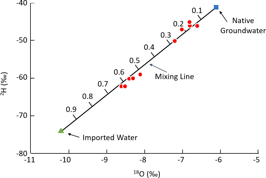
A good example of the use of environmental tracers to determine mixing fractions is provided by a study of artificial recharge in the Santa Clara Valley, California (Figure 12; Muir and Coplen, 1981; Coplen et al., 2000). Groundwater use in the Santa Clara Valley led to groundwater depletion, and an aqueduct was created to import water from northern California. The imported water was discharged into streambeds and percolation ponds to artificially recharge the groundwater. A study subsequently took place to determine the spread of the imported water from the sites where it was introduced, and its contribution to groundwater pumped by downstream wells. The δ ²H and δ ¹⁸O composition of native groundwater was determined to be -41 ‰ and -6.1 ‰, respectively, based on groundwater samples collected in areas unaffected by imported water. The mean value of imported water was -74 ‰ and -10.2 ‰ for δ ²H and δ ¹⁸O, respectively. Groundwater samples downstream of the artificial recharge sites ranged between -45 and -62 ‰ for δ ²H and -6.6 and -8.6 ‰ for δ ¹⁸O, and thus were intermediate between the native groundwater and imported water values (Figure 13). The authors used Equation 8 to estimate the contribution of imported water to downstream wells at between 10 and 70 percent. Lower fractions of imported water were estimated for wells furthest from the artificial recharge sites, with fractions between 10 and 20 percent recorded for wells up to 4 – 5 km downgradient.

Map showing location of Santa Clara Valley, California, USA — **Figure 12** – Location of Santa Clara Valley, California, USA, which has been importing water to recharge local aquifers since the 1960s. Stable isotope studies have been used to evaluate the performance of these managed aquifer recharge schemes (Figure 13). The map on the left shows the location of the inset, on the right.

Graph showing mixing between native groundwater from different sources. — **Figure 13** – Mixing between native groundwater in the Santa Clara Valley, California (blue square) and imported water from northern California (green triangle) that was artificially recharged through streams and percolation ponds. Groundwater downstream of the areas of artificial recharge (red circles) had a stable isotope composition between the two end-members. Numerals indicate the fraction of imported water in the downstream wells. Based on the δ ¹⁸O and δ ²H composition, the contribution of northern California water in downstream wells varies between 10 and 70 percent, with lower values calculated for wells that are furthest from the artificial recharge sites. Based on data in Muir and Coplen (1981) (Cook, 2020).

License