
2.6 Gases in Groundwater: Excess Air
Groundwater samples frequently have higher dissolved gas concentrations than predicted by equilibrium solubility using Henry’s Law (Andrews & Lee, 1979; Herzberg & Mazor, 1979). Groundwater age dating using dissolved gases depends critically on quantifying all processes that lead to measured dissolved gas concentrations. Heaton and Vogel (1981) coined the term excess air because the composition of the excess gas was like the composition of the atmosphere. For low solubility gases such as [latex]He[/latex], [latex]Ne[/latex], and [latex]{SF}_{6}[/latex], excess air can be greater than equilibrium solubility, and hence must be considered for age dating.
Heaton and Vogel (1981) suggested that small bubbles trapped in recharging groundwater might be transported to depth and then completely dissolve. However, a physically more plausible explanation for excess air is a rising water table that does not completely displace the air in what was—prior to the water table rise—the unsaturated zone. The occurrence of bubbles near the water table is discussed in the soil physics literature (e.g., Peck, 1969) and has been shown to reduce the hydraulic conductivity of unconfined aquifers in a zone near the water table (Ronen et al., 1989).
The concept of a rising water table that traps air bubbles that then either partially or fully dissolve due to the increase in fluid pressure is the basis for the widely used closed‑system equilibration (CE) model proposed by Aeschbach‑Hertig and others (2000). The amount of excess air in groundwater depends on the properties of the porous medium (e.g., pore throat size and distribution) and the magnitude of water table rise. Furthermore, the impact of excess air on gas concentrations is generally greatest for low‑solubility gases, especially if the water table rise is sufficient to completely dissolve trapped air bubbles. Dissolved [latex]Ne[/latex] concentration ranging from 10 to 50 percent above solubility are common; however, values exceeding 400 percent of solubility have been measured and may be associated with artificial recharge (Cey et al., 2008).
[latex]Ne[/latex]’s low solubility and its lack of significant subsurface sources makes it a useful indicator of excess air. A common metric of excess air is the deviation of the [latex]Ne[/latex] concentration from the theoretical solubility value, known as ∆[latex]Ne[/latex] defined as shown in Equation (8).
| [latex]\Delta Ne = \frac{C_{m,Ne} - C_{sol,Ne}}{C_{sol,Ne}} \times 100\%[/latex] | (8) |
|---|
where:
| Cm,Ne | = | measured concentration of dissolved [latex]Ne[/latex] (L3M-1, typically in ccSTP/g) |
|---|---|---|
| Csol,Ne | = | theoretical concentration of [latex]Ne[/latex] in equilibrium with the atmosphere (L3M-1, typically in ccSTP/g) |
The computation of Csol,Ne requires assumptions regarding the temperature and atmospheric pressure (elevation) when the sample equilibrated with the atmosphere. Although the temperature may not be known with certainty, the temperature dependence of [latex]Ne[/latex] solubility is relatively small, making ∆[latex]Ne[/latex] a relatively robust indicator of excess air. Because the magnitude of excess air is related to the magnitude of water table rise, ∆[latex]Ne[/latex] has been used as an indicator of both modern and paleo recharge events, that is, to measure the frequency and magnitude of recharge events (Beyerle et al., 2003).
When the elevation of the water table—where groundwater is last in contact with the atmosphere—is relatively well known (i.e., in non‑mountainous terrains), the primary factors affecting the dissolved concentration of atmospheric gases are temperature and the amount of excess air. High solubility gases such as [latex]Xe[/latex] are highly sensitive to temperature but less sensitive to excess air. In contrast, low solubility gases such as [latex]Ne[/latex] are highly sensitive to excess air and less sensitive to temperature. As such, a graphical approach for evaluating temperature and excess air by plotting the dissolved [latex]Xe[/latex] versus [latex]Ne[/latex] concentration is illustrated in Figure 5.
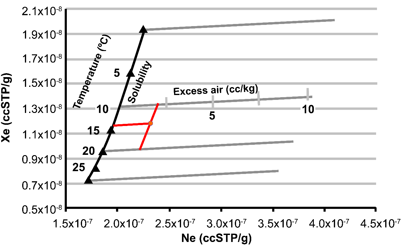
Figure 5 ‑ Graphical approach for evaluating recharge temperature and excess air using [latex]Ne[/latex] and [latex]Xe[/latex] concentration. The solid black line (Solubility) shows the [latex]Xe[/latex] and [latex]Ne[/latex] concentrations expected from solubility equilibrium at various temperatures. The gray lines show expected concentrations if various amounts of excess air are added. The gray lines have been computed for recharge temperatures of 0, 10, 20, and 30 °C. The red circle is a hypothetical sample having [latex]Xe[/latex] and [latex]Ne[/latex] concentrations of 1.18×10⁻⁸ and 2.30×10⁻⁷ ccSTP/g. The sample has an approximate recharge temperature of 14 °C that was obtained by extending a line that is parallel to the gray curves to intersect the black solubility curve, and approximately 2 cc/kg excess air that was obtained by extending a line parallel to the black solubility curve to intersect the gray excess air curve (redrawn from Aeschbach‑Hertig & Solomon, 2013).
The graph shown in Figure 5 was prepared by calculating the solubility concentrations of [latex]Xe[/latex] and [latex]Ne[/latex] at a given atmospheric pressure (e.g., the pressure at the water table where recharge occurred) at various temperatures to form the black solubility curve. For recharge temperatures of 0, 10, 20, and 30 °C, various amounts of excess air were added. The curves in Figure 5 were calculated using Equation (9).
| [latex]C_{i} = \frac{\left( P - e(T) \right)x_{i}}{K_{w,i}(T,S)} + A'x_{i}[/latex] | (9) |
|---|
where:
| A’ | = | amount of excess air in units consistent with Ci (e.g., ccSTP/g) |
|---|
All other parameters are as defined in Equation (4). The first term in Equation (9) is the equilibrium solubility concentration for the ith gas and the second term represents the contribution of the ith gas from excess air. Figure 5 illustrates how the dissolved concentration of [latex]Xe[/latex] depends mostly on temperature, whereas the dissolved [latex]Ne[/latex] concentration depends mostly on the amount of excess air.
The second term in Equation (9) represents a simple model for excess air and was first proposed by Andrews and Lee (1979). This model is known as the unfractionated air (UA) model as it assumes that bubbles are completely dissolved and hence gas is added in using atmospheric proportions rather than solubility proportions. Exercise 1⮧ provides an opportunity to practice determining the fraction of a gas in air‑saturated water.
While the UA model is still widely used and is a useful starting point for evaluating excess air, numerous other models have been proposed. The closed-system equilibration (CE) model introduced by Aeschbach‑Hertig and others (2000) describes bubbles trapped from a rising water table that may not fully dissolve if there is insufficient fluid pressure. The partial dissolution of bubbles leads to a fractionation of the dissolved gases between the groundwater and the bubbles according to the solubility of gases. The CE model has two parameters, one that describes the volume of gas trapped per unit mass of water (A) and another for the fractionation factor (F) that describes the fraction of the original gas volume in the porous medium that does not dissolve. The equation for computing the dissolved gas concentration using the CE model is shown in Equation (10).
| [latex]C_{i} = \frac{\left( P - e(T) \right)x_{i}}{K_{w,i}(T,S)} + \frac{(1 - F)Ax_{i}}{1 + \frac{FAx_{i}}{\frac{\left( P - e(T) \right)x_{i}}{K_{w,i}(T,S)}}}[/latex] | (10) |
|---|
where:
| A | = | volume of gas trapped in the porous media per unit mass of water (L3M-1, typically in ccSTP/g) |
|---|---|---|
| F | = | fractionation factor (dimensionless) |
The parameter A in the CE model should not be confused with A’ in the UA model, although they both have dimensions of volume of gas per mass of water. In the case of the UA model, A’ represents the volume of air that dissolves into the water, whereas A in the CE model is the volume of air per unit mass of water that exists in the porous medium before gas dissolution. When F equals 0 (i.e., none of the original gas volume remains in the porous medium), all the available gas dissolves, in which case A’ equals A, and the CE model is the same as the UA model.
The CE model provides a physically more plausible description of gas dissolution than the UA model because very large water table rises are required to produce sufficient pressure to fully dissolve the amount of excess air that is often observed in groundwater samples. However, the CE model has an additional parameter that must be determined, and its evaluation is not possible with the simple graphical approach shown in Figure 5. An optimization procedure for determining both A and F as well as the recharge temperature is discussed later in this section.
Numerous additional models have been proposed to describe the occurrence of excess air in groundwater. These include:
- a partial re‑equilibration (PR) model (Stute et al., 1995),
- a multi‑step partial re‑equilibration (MR) model (Kipfer et al., 2002),
- a partial degassing (PD) model (Lippmann et al., 2003),
- a negative pressure (NP) model (Mercury et al., 2004),
- an oxygen depletion (OD) model (Hall et al., 2005), and
- a gas diffusion relaxation (GR) model (Sun et al., 2008).
These models are discussed in Aeschbach‑Hertig and Solomon (2013).
Subsurface processes that lead to excess air are complex and none of the models fully describe these and their associated kinetics. The CE model generally provides a reasonable description of excess air for the purpose of groundwater dating, but site‑specific processes may be better described by one of the other models.
The graphical approach (Figure 5) for evaluating recharge temperature and excess air is useful for the UA model when the concentration of two gases (e.g., [latex]Xe[/latex] and [latex]Ne[/latex]) have been measured and there are two unknowns. However, when an excess air model with more parameters is used, more concentration measurements are needed as well as a systematic technique for estimating these parameters. The inverse determination for excess air parameters was simultaneously introduced by Ballentine and Hall (1999) and Aeschbach‑Hertig and others (1999) and involves choosing parameters (e.g., T, A, F) such that the sum of the error‑weighted deviations between measured and simulated gas concentrations, known as chi‑squared ([latex]X^{2}[/latex]), is minimized. The simulated concentrations come from models such as shown in Equation (10) that depend on temperature, salinity, pressure or elevation, and excess air parameters. Mathematically, [latex]X^{2}[/latex] is expressed as shown in Equation (11).
| [latex]X^{2} = \sum_{i = 1}^{n}\left( \frac{C_{m,i} - C_{s,i}}{\sigma_{i}} \right)^{2}[/latex] | (11) |
|---|
where:
| [latex]C_{m,i}[/latex] | = | measured concentration of the ith gas (L3M-1, typically in ccSTP/g) |
|---|---|---|
| [latex]C_{s,i}[/latex] | = | simulated concentration of the ith gas (L3M-1, typically in ccSTP/g) |
| [latex]\sigma_{i}[/latex] | = | measurement error of the ith gas (L3M-1, typically in ccSTP/g) |
The inverse approach uses powerful optimization algorithms to iteratively select values of unknown parameters in an excess air model until [latex]{\ X}^{2}[/latex] reaches a minimum value—that is, when the average deviation between simulated and measured values is minimized. By weighting the deviations by the measurement errors ([latex]\sigma_{i}[/latex]), it is possible to evaluate the probability that the chosen excess air model provides an adequate representation of the solubility and excess air processes. For example, if four gases are measured (i.e., [latex]i\ = \ 4[/latex] in Equation (11)) and the difference between each measured gas concentration ([latex]C_{m,i}[/latex]) and the concentration computed ([latex]C_{s,i}[/latex]) using an excess air model was equal to the measurement error ([latex]\sigma_{i}[/latex]), then [latex]{\ X}^{2}[/latex] would equal 4.
If our excess air model included three unknown parameters (e.g., T, A, F), then the degrees of freedom (DF) would be 1 (DF = constraints = free parameters = number of gases measured [latex]-[/latex]number of unknown parameters = 4 [latex]-[/latex]3 = 1). The probability (p‑value) for a [latex]{\ X}^{2}[/latex] of 4 can be computed to be 0.046 (from standard [latex]{\ X}^{2}[/latex] probability calculators or tables). High [latex]{\ X}^{2}[/latex] values give low p‑values. This means there is approximately a five percent chance that the [latex]{\ X}^{2}[/latex] value results from random measurement errors.
In general, p‑values of less than 0.01 have been used for rejecting a given excess air model, and thus we cannot reject the possibility that the model itself in our example is inappropriate. On the other hand, a [latex]{\ X}^{2}[/latex] value of 7 with 1 DF would have a p‑value of 0.008. Since there is less than a one percent chance that this [latex]{\ X}^{2}[/latex] value results from random measurement errors, it is probably not an adequate description of the physical processes for that sample—if the measurement error used for calculating [latex]{\ X}^{2}[/latex] is correct.
The [latex]{\ X}^{2}[/latex] probability distribution was developed for hypothesis testing and is best used for rejecting a given model rather than finding the “best” model. In other words, if two models are compared, the one with the highest [latex]{\ X}^{2}[/latex] is not necessarily “worse” than the model with a lower [latex]{\ X}^{2}[/latex] if both have p‑values that are greater than 0.01. In such a case, the choice between models should rely on which model provides a better physical description of subsurface processes at a given site. Exercise 2⮧ provides further practice with the [latex]{\ X}^{2}[/latex] concept.
The inverse approach for noble gases has been implemented into several computer programs. Several of these use Excel workbooks with solubility equations as a function of temperature and pressure and excess air models programmed into worksheets. Table 3 shows known programs along with their availability.
While excess air in groundwater can clearly result from natural processes such as water table fluctuations, it is important to be aware that it can also be an artifact of drilling operations such as using air as a drilling fluid or well development using compressed air. If air bubbles are forced into the formation many borehole volumes must be purged to eliminate this artifact (Manning et. al., 2003; Poulsen et al., 2020).
Table 3 ‑ Software available for interpreting dissolved gases.
| Program name | Description | Availability | Comments |
|---|---|---|---|
| NOBLEBOOK | Excel workbook for inverse modeling of dissolved noble gas concentration | Uses Solver™ in Excel for optimization. | |
| PANGA | Computer program for the analysis of noble gas data. | Includes uncertainty analysis. Versions available for both Windows and Mac OS | |
| DGMETA | Excel based computer program for dissolved gas modeling and environmental tracer analysis | Includes uncertainty analysis and SF6 and CFCs |