
3.4 Calculation of Tracer Age
When the recharge concentration increases monotonically with time or is stable, the age of a radioactive transient tracer can be calculated as previously discussed by correcting the measured concentration for decay and projecting the decay‑corrected value back to its intersection with the recharge versus time curve. However, when the recharge concentration declines with time, a unique determination of age is not always possible. If the recharge concentration declines at the same rate as the tracer decays, an infinite number of possible ages can explain the measured value. The non‑uniqueness in age is illustrated in Figure 10 which shows the atmospheric [latex]_{}^{3}H[/latex] values for Vienna, Austria, along with decay curves for three hypothetical samples collected in 2015.
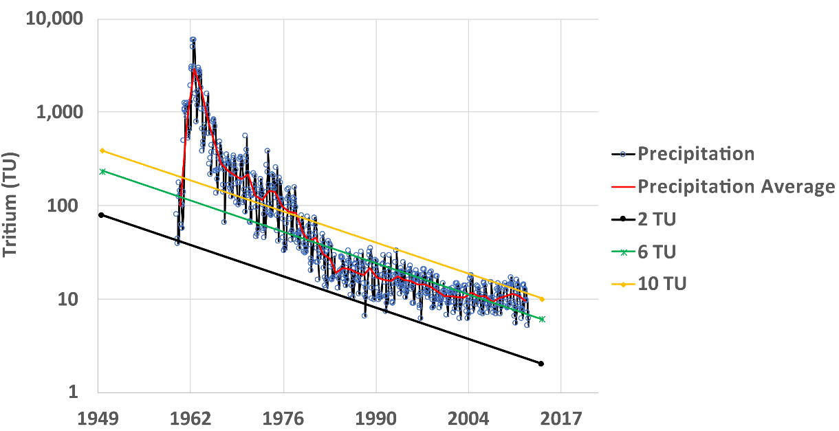
Figure 10 ‑ Example of groundwater dating with [latex]_{}^{3}H[/latex] with three hypothetical samples collected in 2015 in the vicinity of Vienna, Austria, where the precipitation data were collected. The 2 TU sample can be reasonably assigned a recharge year of 1961. The decay curve for the 6 TU sample intersects the average precipitation curve (solid red line) in 1961 and a few times between 1982 and 2009, so only a minimum age of six years (2015 – 2009 =[latex]6[/latex]) can be assigned by using the latest time at which the decay curve crosses the average precipitation curve. The 10 TU sample is likely modern (age = 0), but recharge years of 1962 and 1978 cannot be ruled out.
The red curve in Figure 10 represents annual average values and may be a more representative value for recharge at the water table with dispersion in the unsaturated zone smoothing annual variations. Sample 1 has a measured concentration of 2 TU, and this sample can reasonably be interpreted as being recharged prior to the bomb peak, most likely in the early 1960s. Although the decay curve for this sample intersects the precipitation curve for one sample on October 15th, 1988, it is unlikely this single value was representative of recharge in 1988; it is more likely that the average value was around 14 TU in 1988. If the pre‑bomb recharge concentration is assumed to be 10 TU for this location, then the most probable recharge year for this sample is about 1960 for an age of 2015 – 1960 = 55 years.
Hypothetical sample 2 has a concentration of 6 TU, and its decay curve intersects the average precipitation curve in 1961 and a few times between 1982 and 2002. With the assumption that unsaturated zone transport has smoothed the annual variations in precipitation, it is reasonable to conclude that this sample has a minimum age of 6 years (2015 – 2009 =[latex]6[/latex]), but it could be as old at 55 years (2015 – 1960 =[latex]55[/latex]).
The third sample is likely modern with an age of zero, but its decay curve intersects the average precipitation curve in 1962 and 1978, so older ages cannot be ruled out.
The procedure used for the previous example can be summarized in the following four steps:
- Obtain an atmospheric [latex]_{}^{3}H[/latex] input function for the area of interest, which can be challenging. For study sites near a GNIP station, missing data points—a common occurrence—can be filled in using a linear regression with one of the complete stations such as Vienna, Austria, or Ottawa, Canada. For study sites not near a GNIP station, the input function might be reconstructed by triangulation or inverse distance weighting of the correlation parameters of nearby stations (Harms et al., 2016; Michel et al., 2018). For sites located in the USA, the correlation and spatial interpolation of Michel and others (2018) might be used. The global model of Terzer‑Wassmuth and others (2022) may be especially useful for estimating the contemporary value.
- Compute annual average concentrations. If precipitation amount data are available, the monthly values should be weighted by precipitation.
- Calculate the decay curve for a given sample. The sample date and measured concentration represent one point for this curve and only one additional point is needed. The additional point can be calculated using Equation (12).
| [latex]C_{o} = C_{m}\exp(\lambda\Delta t)[/latex] | (12) |
|---|
where:
| [latex]C_{o}[/latex] | = | concentration at an arbitrary time; a convenient choice is 1950 as the precipitation [latex]_{}^{3}H[/latex] record begins after 1950 (e.g., TU) |
|---|---|---|
| ∆t | = | sample time – Co time (T) |
| [latex]C_{m}[/latex] | = | sample concentration (e.g., TU) |
| [latex]\lambda[/latex] | = | tritium decay constant (T-1, 0.05626 yr–1) |
- Plot the raw [latex]_{}^{3}H[/latex] in precipitation data, the average (precipitation weighted) data, the sample concentration ([latex]C_{m}[/latex]) and the arbitrary [latex]C_{o}[/latex] data, with a line connecting [latex]C_{o}[/latex] and [latex]C_{m}[/latex].
The previous example illustrates the variable degree to which a unique age can be assigned to a sample. Even if a unique age cannot be assigned, it may be possible to calculate a minimum age using Equation (13).
| [latex]{Age}_{\min} = \frac{- \ln\left( \frac{C_{meas}}{C_{background}} \right)}{\lambda}[/latex] | (13) |
|---|
where:
| [latex]{Age}_{\min}[/latex] | = | minimum age of the sample (T) |
|---|---|---|
| [latex]C_{background}[/latex] | = | [latex]_{}^{3}H[/latex] concentration in precipitation at the time the sample was collected (e.g., TU) |
| [latex]C_{meas}[/latex] | = | sample concentration (e.g., TU) |
| [latex]\lambda[/latex] | = | tritium decay constant (T-1, 0.05626 yr–1) |
[latex]C_{background}[/latex] in Equation (13) is the [latex]_{}^{3}H[/latex] concentration in precipitation at the time the sample was collected and assumes that previous atmospheric [latex]_{}^{3}H[/latex] values were greater than or equal to [latex]C_{background}[/latex]. Furthermore, [latex]C_{meas}[/latex] must be less than [latex]C_{background}[/latex]. In practice, Equation (13) generally applies only to samples collected after about the year 2000 and in areas with no significant local [latex]_{}^{3}H[/latex] sources. Exercise 3⮧ provides an opportunity to practice estimating sample age.
When a vertical profile of [latex]_{}^{3}H[/latex] values is available, it is sometimes possible to identify the mid‑1960s bomb peak as an event marker, although decay and dispersion are making it harder to locate the peak as time goes on. This technique has more commonly been used in the unsaturated zone but has also been used in the saturated zone. Figure 11 shows a vertical profile of [latex]_{}^{3}H[/latex] values from a shallow unconfined aquifer near Sturgeon Falls, Ontario, Canada (Solomon et al., 1993). The 1963 bomb peak is clearly delineated in the profile and defines the age of groundwater at the depth and location of the peak.
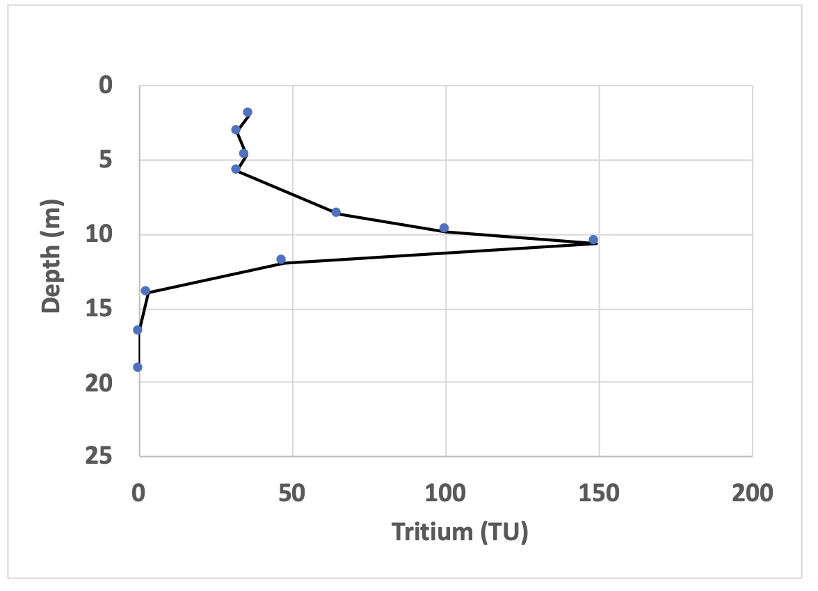
Figure 11 ‑ Vertical profile of [latex]_{}^{3}H[/latex] values from an unconfined aquifer near Sturgeon Falls, Ontario, Canada (redrawn from Solomon et al., 1993). Peak [latex]_{}^{3}H[/latex] concentration at a depth of 10.6 meters marks the location of water that recharged in 1963.
While the determination of groundwater age from a single discrete sample using [latex]_{}^{3}H[/latex] can be non‑unique as described previously, a unique determination of the mean residence time may be possible using a lumped parameter model (LPM; Maloszewski & Zuber, 1982). The details of LPMs are beyond the scope of this book, but as shown by Morgenstern and Taylor (2009), if a sample can be collected that contains a flow‑weighted mixture of all aquifer flow paths—using a fully‑screened well or at a major spring where flow paths converge—and if the residence time distribution is known, it may be possible to uniquely define the mean residence time from this single, or mixed, sample. Prior understanding of site conditions and conceptual models are required for this approach to be successful.