Solution Exercise 7
The solution to Exercise 7 is in two parts: a) and b).
- We first solve for the mole fraction of [latex]{SF}_{6}[/latex] that would be in equilibrium with the measured concentrations at a temperature of 15 °C and elevation of 800 m. This was shown in Equation (25) for UA as shown here.
[latex]x = \frac{C}{K_{h}(P - e) + A'}[/latex]
We need to first compute P at 800 m, e at 15 °C, and Kh at 15 °C. P is calculated as shown here.
[latex]P = P_{0}\exp\left( - \frac{Z}{Z_{s}} \right) = 1\ atm\ exp\left( - \frac{800\ m}{8300\ m} \right)\ = \ 0.908\ atm[/latex]
e at 15 °C is calculated and converted to atmospheres as shown here.
[latex]e = 10^{A\ - \ \frac{B}{C + T}} = 10^{\left( 8.07131 - \ \frac{1730.63}{233.426 + 15} \right)} = 12.73\ mmHg\ \frac{1atm}{760\ mmHg} = 0.0167\ atm[/latex]
Table 6 gave [latex]K_{h}[/latex] values at 10 °C and 20 °C but not at 15 °C. We could use the empirical equations of Bullister and others (2002), or we can linearly interpolate between 10 °C and 20 °C as shown in the following equations.
[latex]\ K_{h}\ at\ 15\ {^\circ}C\ = \ K_{h}\ at\ 10\ {^\circ}C\ + \frac{(15\ {^\circ}C - 10\ {^\circ}C)}{(20\ {^\circ}C - 10\ {^\circ}C)}\ \left( K_{h}\ at\ 20\ {^\circ}C\ - \ K_{h}\ at\ 10\ {^\circ}C \right) = \ 0.0003969\ + \frac{(15\ {^\circ}C - 10\ {^\circ}C)}{(20\ {^\circ}C - 10\ {^\circ}C)}(0.0002739\ - \ 0.0003969) = \ 0.0003354\ \frac{mole}{kg\ atm}[/latex]
So, the mole fraction becomes (with [latex]A'\ =[/latex]0) as shown in the following equation.
[latex]x = \frac{2.6x10^{- 15}\ \frac{moles}{kg}}{0.0003354\ \frac{mole}{kg\ atm}(0.908\ atm - 0.0167\ atm) + \ 0}[/latex]
[latex]= 8.70x10^{- 12}[/latex]
[latex]= 8.7\ pptv[/latex]
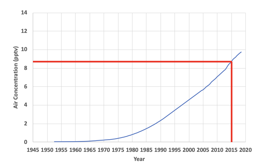
Next the atmospheric curve shown in Figure 20 is utilized to find the year that the atmosphere had a mole fraction (essentially equal to the mixing ratio) of 8.7 pptv as shown below. This is approximately 2015. Since the sample was collected in 2018, it has an apparent tracer age of 2018 – 2015 = 3 years.
- To add 0.003 ccSTP/g = 3.0 ccSTP/kg of excess air, we must convert ccSTP/kg to moles/kg. Equation (3) showed this conversion as duplicated here.
[latex]n = \frac{PV}{RT} = \frac{(1\ atm)(ccSTP)}{82.05746\ \frac{ccSTP\ atm}{K\ mole}(273.15\ K)}\ = \ \frac{1\ atm\ \left( 3.0\ \frac{ccSTP}{kg} \right)\ }{82.05746\ \frac{ccSTP\ atm}{K\ mole}(273.15\ K)}\ = \ 0.000134\ \frac{moles}{kg}[/latex]
With excess air, Equation (25) can be used to calculate the mole fraction of [latex]{SF}_{6}[/latex] in the atmosphere that would have resulted in the measured concentration. This is duplicated here.
[latex]x = \frac{2.6x10^{- 15}\ \frac{moles}{kg}}{0.0003354\ \frac{mole}{kg\ atm}(0.908\ atm - 0.0167\ atm) + \ 0.000134\ \frac{moles}{kg}}[/latex]
[latex]= 6.01x10^{- 12} = 6.01\ pptv[/latex]
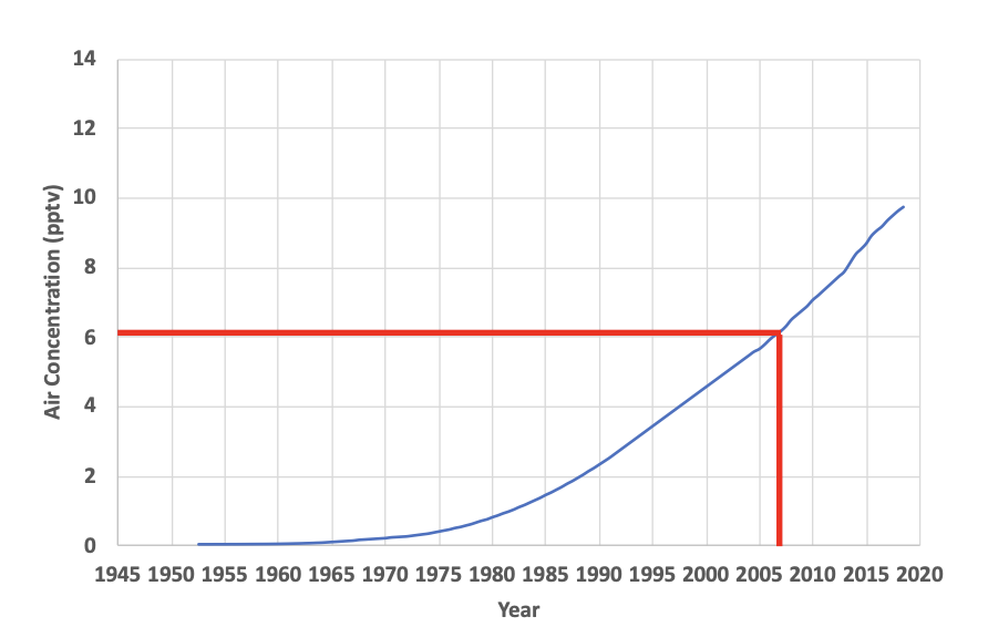
Then the atmospheric curve in Figure 20 is utilized to find the year that the atmosphere had a mole fraction (essentially equal to the mixing ratio) of 6.01 pptv as shown below. This is approximately 2006.5. Since the sample was collected in 2018, it has an apparent tracer age of 2018 [latex]-[/latex] 2006.5 = 11.5 years. This is 8.5 years older than the tracer age when excess air was not included and illustrates the importance of including excess air for calculating [latex]{SF}_{6}[/latex] tracer ages.