4.1 Darcy’s Law
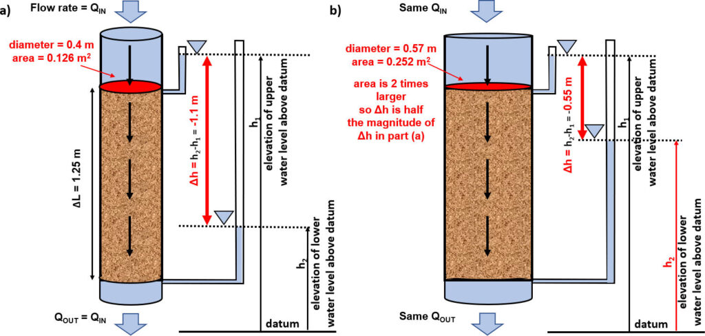
In 1856, Henry Darcy reported results of experiments used to enhance the water flow through sand filter beds used by the city of Dijon, France for water treatment (Darcy, 1856). As an engineer, he wanted to design sand beds that would efficiently and effectively filter the daily volume of water needed by the city. To evaluate the volume of water that could be filtered in a given period of time, Darcy experimented with changing: the type of sand; the area of the filter bed (diameter of the tube in his experiments); the thickness of the sand (length of the sample in his experiments); and, the force driving water through the filter bed (Figure 15).

To determine the driving force, he used mercury manometers to measure pressure in the reservoir on each end of the sand filter because he knew that the combination of water pressure and elevation would describe the mechanical energy at each location.
By conducting a number of experiments under varying conditions, Darcy discovered a mathematical relationship that indicated the steady-state flow rate through the circular sand filter, Q, was: directly proportional to the cross sectional area of the filter, A; directly proportional to the difference in hydraulic head (elevation of water in the piezometers measured from a datum) on each side of the filter, Δh; and inversely proportional to the length of the filter material, ΔL (Equation 14 and Figure 15b). The elevation of the water level in the piezometers is referred to a hydraulic head.
 |
(14) |
where:
| Q | = | volumetric flow rate (L3/T) |
| Δh | = | difference in hydraulic head between two measuring points, h2 – h1, where h2 is head at a location beyond the location of h1 in the direction of flow (L) |
| ΔL | = | length along flow path between locations where hydraulic heads are measured (L) |
| A | = | cross-sectional area perpendicular to the direction of flow (L2) |
The negative sign is included in Equation 14 because the volumetric flow rate, Q, is positive in the direction of flow under a negative change in head (i.e., head decreases in the direction of flow).
By experimenting with coarse- to fine-grained sands, Darcy found that the flow rate was also directly proportional to the character of the sand he placed in the column (Figure 15). The proportionality constant is referred to as the hydraulic conductivity or permeability and its use converts the proportionality to an equivalency. This mathematical relationship is referred to as Darcy’s Law (Equation 15). Darcy’s law is the fundamental equation used to describe the flow of fluid through porous media, including groundwater.
 |
(15) |
where:
| Q | = | volumetric flow rate (L3/T) |
| K | = | hydraulic conductivity, is the proportionality constant reflecting the ease with which water flows through a material (L/T) |
| Δh | = | difference in hydraulic head between two measuring points as defined for Equation 14 (L) |
| ΔL | = | length along the flow path between locations where hydraulic heads are measured (L) |
 |
= | gradient of hydraulic head (dimensionless) |
| A | = | cross-sectional area of flow perpendicular to the direction of flow (L2) |
Consequently, if the area of the column is increased by a factor of two while the flow rate and length of saturated sediment are held constant, the difference in water elevations (Δh) in the piezometers will decrease by a factor of two (Figure 16). It also holds that if the cross-sectional area, flow rate and hydraulic conductivity were constant and the column length (ΔL) is reduced by one half the difference in head (Δh) will decrease by 2.
Darcy’s Law in the most general form is presented as a differential where dh and dL are defined over an infinitesimally small interval, so Equation 15 becomes Equation 16.
 |
(16) |
where:
| dh | = | Δh over an infinitesimal interval (L) |
| dL | = | ΔL over an infinitesimal interval (L) |
Darcy’s Law describes how head, hydraulic gradients and hydraulic conductivity are linked to quantify and describe groundwater flow. For example, to compute the discharge of groundwater (Q) through a cross-sectional area of sand below the water table that is 100 m by 30 m (A) with a hydraulic conductivity of 15 m/d (K), and with a head change (Δh) of -2 m over a flow path length (ΔL) of 1000 m, Equation 15 is applied. The discharge is calculated as follows.
 |
Specific Discharge
Darcy’s law can also be represented in terms of specific discharge, a flux, which is discharge per unit area (q) as shown in Equation 17.
 |
(17) |
where:
| q | = | specific discharge in the direction of flow (L3/L2T) |
Specific discharge is also referred to as “groundwater flux” and has units of L3/(L2T) which is discharge per unit area, or simply L/T (Figure 17a). It is also referred to as Darcy flux, Darcy velocity, and apparent velocity. It represents the volume of water that flows through a unit cross sectional area of porous media per unit time. The apparent velocity term is sometimes used because by cancelling L2 of the flux units, the units become L/T, which are velocity units. However, this is not a true groundwater velocity, it is a flux. It is best to always use flux units (L3/(L2T)) when reporting specific discharge values, or at least to use the term flux or apparent velocity so the meaning will be clear.
To compute the flux of groundwater through the cross-sectional area under the conditions presented in groundwater discharge conditions described above it follows that:
 |
Average Linear Velocity
In contrast to the apparent velocity portrayed by specific discharge (Figure 17a), Darcy’s Law can also be used to derive the actual rate at which water is flowing through a cross sectional area of porous media, the groundwater velocity. The groundwater velocity, v, is higher than the specific discharge because the water can only pass through the portion of the cross-sectional area that is connected pore space, ne. That cross-sectional area is the product of the area of porous medium and the effective porosity, ne. This velocity is called the average linear velocity, seepage velocity or average interstitial velocity, and it is the flux, q, divided by the effective porosity, ne, q/ne = v (Figure 17b).

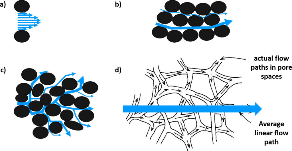
The concept of “actual” groundwater velocity, recognizes that microscopic velocities within the complex interconnected pore structure are variable and difficult to characterize (Figure 18a, b, and c). In addition to the variability of flow trajectory (Figure 18c), the microscopic velocities also vary because the pore throats and channels are variable (Figure 18a and b). Thus, the overall effect of groundwater flowing in a lattice work of varied pore channels is more easily represented by a composite groundwater velocity value, the average linear velocity for a representative elementary volume of porous material (Figure 18d and Figure 17b). The average linear velocity in the direction of flow is attained by considering the volumetric flow rate per unit area of porous medium divided by the effective porosity, ne, using any of the forms of Equation 18.
 |
(18) |
The average linear velocity is a vector that represents the average direction and magnitude of the ensemble of water particles flowing through the porous medium as shown by the large arrow in Figure 18d. It does not represent the velocity in microscopic individual pore channels. Such velocities are highly variable and contribute to dispersion of dissolved constituents in groundwater systems.
When the volumetric flow rate is known, the average linear velocity can be computed using estimates of the flow area and effective porosity. If the effective porosity is 0.13 and the conditions as described in the specific discharge calculation above are applied, then the average linear velocity would be:
 |