7.2 Governing Equations for Confined Transient Groundwater Flow
The law of conservation of mass for flow through a saturated porous medium requires that the flux of fluid mass into the volume equals the flux of fluid mass out of the volume plus the change in mass stored within the volume. Darcy’s Law is represented by the specific discharge, q. The mass flux is ρ q (Equation 52).
| Mass Flux = ρ q | (52) |
where:
| Mass Flux | = | mass of water passing through a unit area per unit time (M/(L2T)) |
| ρ | = | density of water (M/L3) |
| q | = | specific discharge (L/T) |
One-dimensional Flow
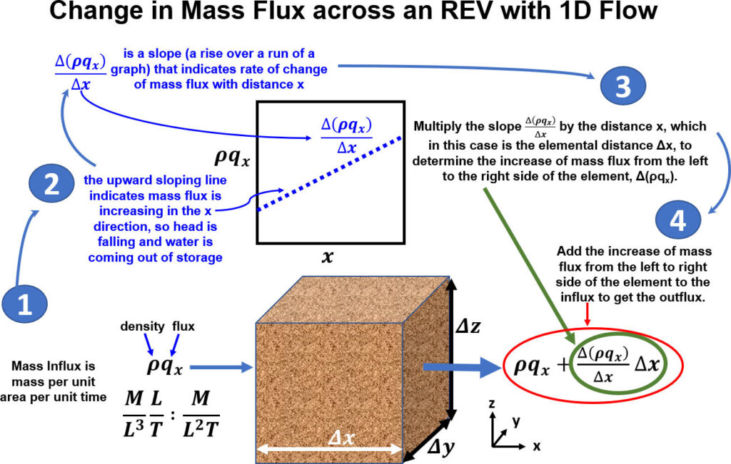
Governing equations describing groundwater flow are most often presented as representing steady state or transient conditions, and flow in two- or three-dimensional space. However, especially for readers who are not as familiar with differential equations, it is useful to consider one-dimensional flow (along the x axis) through a REV first (Figure 52). The mass flux into the REV is the product of the specific discharge and the fluid density (item 1 of Figure 52). If the head is declining, then water is coming out of storage from the porous medium and the mass flux will increase across the REV as shown in item 2 of Figure 52. Multiplying the slope of the mass-flux-vs-distance graph by the distance across the REV (Δx) determines the increase in mass flux from left to right (item 3 of Figure 52). Adding that increase of flux across the element to the influx produces the outflux (item 4 of Figure 52). It is useful to recall that a flux has units of velocity (L/T) because it is a flow rate L3/T divided by the area of flow (L3/T)/(L2).
The fluxes in and out of the element in Figure 52 are shown in Equations 53 and 54 respectively.
Mass Flux In =  |
(53) |
Mass Flux Out =  |
(54) |
where:
| Mass Flux | = | mass of water passing through a unit area per unit time (M/ (L2T)) |
| ρ | = | density of water (M/L3) |
| qx | = | specific discharge (L/T) |
| Δx | = | length of the elementary volume in the x direction (L) |
Mass flow rate is obtained by multiplying the fluxes by the cross-sectional area of the elementary volume that they pass through (for one-dimensional flow in the x direction, the area is ΔyΔz), as in Equations 55 and 56.
Mass Flow In =  |
(55) |
Mass Flow Out =  |
(56) |
where:
| Mass Flow | = | mass of water passing into, or out of, an REV per unit time (M/T) |
| Δy, Δz | = | length of the elementary volume in the y and z directions (L) |
Next, the change in the inflow is examined using and analysis of the inward flow of mass. The inward flow of mass is defined as mass inflow minus outflow, a positive value of inward flow of mass indicates that the inflow exceeds the outflow and water is going into storage, while a negative value indicates outflow exceeds inflow and water is coming out of storage. The inward flow of mass is determined by subtracting the outflow (Equation 56) from the inflow (Equation 55) as shown in Equation 57.
Inward Flow of Mass =  |
(57) |
where:
| Inward flow of Mass | = | mass of water flowing into the elementary volume per unit time (M/T) |
Expanding the second term of Equation 57 and subtracting yields Equation 58. The negative sign indicates that water is coming out of groundwater storage, thus inward flow of mass is negative.
Inward Flow of Mass =  |
(58) |
Given that the inward flow of mass is the increase in mass in the element per unit time and mass must be conserved, then the inward mass flow per unit time must equal the change in mass storage per unit time. Recall that specific storage is the change in volume of water stored in a unit volume of aquifer for a change in head, so the change in volume with time is shown as Equation 59.
 |
(59) |
where:
| ΔV | = | change in volume of water in the REV (L3) |
| ρ | = | density of water in the REV (M/L3) |
| g | = | gravitational constant (acceleration of gravity) (L/T2) |
| α | = | compressibility of the aquifer solid structure (L3/L3)/(F/L2), inverse pressure) |
| β | = | compressibility of water (L3/L3)/(F/L2), inverse pressure |
| n | = | fully connected total porosity (ne) of the REV (dimensionless) |
The change in stored mass for a unit of time is obtained by the product of Equation 59 and the water density (Equation 60).
 |
(60) |
where:
| ΔM | = | change in mass of water in the REV (M) |
Equating the change in mass storage (Equation 60) with the inward flow of mass (Equation 58) produces Equation 61.
 |
(61) |
Although it is recognized that the water density changes slightly in response to head changes (i.e., pressure changes), the amount of compression or expansion is small enough to assume constant density for the vast majority of applications so, ρ, can be taken out of the delta-term due to its minimal change with time (Equation 62).
 |
(62) |
Dividing both sides by ρ and by Δx Δy Δz , then substituting the specific storage, Ss, for ρg(α + nβ) provides Equation 63.
 |
(63) |
The specific discharge can be represented by Darcy’s Law, where qx = – KxΔh/Δx, assuming the principal direction of the component of hydraulic conductivity is aligned with the x-axis, as represented in Equation 64.
 |
(64) |
The Δ’s in the equation describe discrete changes across a small elementary volume. This allows translation of this relationship into a differential form when the discrete change is infinitesimal by replacing Δ with d, providing the derivative of a smooth function (Equation 65).
 |
(65) |
Equation 65 is the governing equation for confined, one-dimensional, transient, heterogeneous conditions of groundwater flow. Equation 65 can also be written as Equation 66.
 |
(66) |
Three-dimensional Flow
In most cases, the flux will not be one-dimensional along the x-axis. It will occur in an arbitrary direction with a component in each of the x, y, and z directions (see for example Section 5.4), thus the change in mass flux across the element needs to be accounted for in each of the three-dimensions as shown in Figure 53. The partial differential symbol (∂/∂x) is used in order to represent that only a part of the change in flux across the element occurs in the x direction, as there are also changes in the y– and z-directions (∂/∂y, ∂/∂z); and when the system is transient, with time, ∂/∂t. The groundwater flow equation for three-dimensional flow is the same as the equation for one-dimensional flow with additional flux terms for the y– and z-directions.

Confined, three-dimensional, transient, anisotropic, heterogeneous conditions of groundwater flow are represented by Equation 67.
 |
(67) |
When the values of Kx, Ky and Kz are constants (but not the same value) they can be taken out of the derivative resulting in Equation 68. It describes confined, three-dimensional, transient, anisotropic, homogeneous conditions of groundwater flow.
 |
(68) |
For confined, three-dimensional, transient, isotropic and homogeneous conditions of groundwater flow, Kx = Ky = Kz = K, thus one value of K is sufficient to represent the hydraulic conductivity and Equation 69 is formulated.
 |
(69) |
For confined, two-dimensional (plan view), transient, isotropic, homogeneous conditions in an aquifer of constant thickness, the z-terms for vertical flow can be omitted from Equation 69. Also, saturated thickness, b, is not dependent on head, h, (Figure 54) and assuming the aquifer thickness is constant, both sides of Equation 69 can be multiplied by the aquifer thickness leading to Equation 70 that represents horizontal flow in a map view.

 |
(70) |
Then, by using the definition of transmissivity, T, as Kb and storativity, S, as Ssb, Equation 70 can be written as Equation 71.
 |
(71) |
Equation 70 and Equation 71 represent groundwater flow under confined, two-dimensional (plan view), transient, homogeneous and isotropic conditions using S and T.