4.3 Hydraulic Gradient
As shown in Equation 16, the ratio of ∆h and ∆L (the hydraulic head difference divided by the length of the sample or the distance separating two head locations) can be generalized into a differential called the hydraulic gradient, dh/dl as in Equation 21.
 |
(21) |
where:
| dh | = | ∆h over an infinitesimal interval (L) |
| dl | = | ∆L over an infinitesimal interval (L) |
Given that the hydraulic gradient is computed by subtracting the head, h1, at the origin from the head, h2, at a distance ΔL from the origin in the direction of flow, and then dividing by the distance ΔL, the negative sign in Equation 21 provides a positive value of volumetric flow rate from high to low hydraulic head. In the vertical column shown in Figure 19, the value of head h2 at L2 is subtracted from h1 at L1. This results in a negative gradient, ∆h/∆L. That is, flow proceeds in the down gradient direction. Using this convention, flow is away from h1 and toward h2. With the difference in head being a lower head value minus a higher head value, the gradient is negative (Equation 22).
 |
(22) |
Hydraulic gradient can also be represented in three dimensions when flow is not aligned with a coordinate axis, x, y, or z (Equation 23), so there is a component of flow in each axis direction as shown in Equation 23. In this case, in order to determine the direction of flow, each hydraulic gradient component is calculated with h2 being located at a larger coordinate position than h1.
 |
(23) |
The partial differential (∂) representation (∂\∂x) is used because the gradient is partially dependent on the conditions in each of the coordinate directions. The resulting gradient vector (the overall magnitude and direction of the gradient) is dependent on the magnitudes of all three components of gradient in the x, y, and z directions.
The hydraulic gradient is commonly represented using the letter “i” such that Darcy’s law is often written as shown in Equation 24.
| Q = – KiA | (24) |
where:
| i | = | hydraulic gradient (Δh/ΔL or dh/dl) (dimensionless: L/L) |
The difference in the hydraulic head over a distance along the flow path is defined as the hydraulic gradient, Δh/ΔL. This gradient of mechanical energy is the driving force of groundwater flow. If water is not moving, the gradient is zero, and the value of head is the same everywhere. In this situation, hydrostatic conditions exist. Under hydrostatic conditions the elevation head and pressure head at any location in the porous media combine to form the same hydraulic head value (Figure 24).

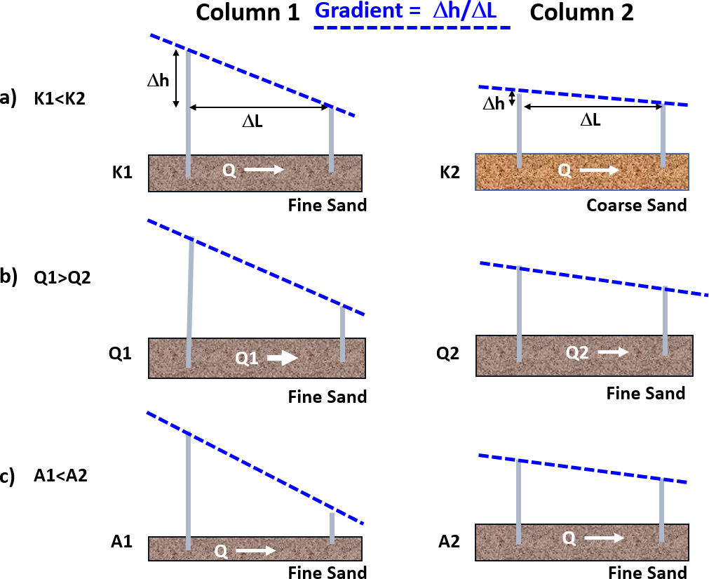
Groundwater flow occurs in the direction of the decreasing head, independent of the position of the porous medium in space (Figure 20). Local gradients are impacted by the magnitude of the hydraulic conductivity, flow rate, and cross-sectional area as stated by Darcy’s Law (Equation 22) and illustrated in Figure 25.
It is important to note that in addition to representations of gradients in the horizontal x,y-plane (e.g., Δh/ΔL as displayed in Figure 22 and Figure 25), vertical gradients, Δh/Δz, in the vertical x,z-plane can be assessed to examine if water is moving upward or downward at a given location (Figure 26). To evaluate vertical gradients, wells or piezometers extending to different depths are completed immediately adjacent to each other or are vertically isolated from one another in a single borehole. The magnitude of the vertical gradient is computed by comparing the absolute value of the head difference between the piezometers in the direction of flow, Δh = | hB – hA |, over the vertical distance separating their measurement locations, ΔL = | ZB – ZA |. If piezometers or monitoring wells have screens open to the groundwater over an interval, the measuring point is designated as the midsection of the screened interval. The direction of the gradient is determined by comparing the head in the shallow piezometer, A, with that of the deeper piezometer, B. In Figure 26, the head at B is less than the head at A, so flow is downward. If the head in B was higher than A then the gradient would be upward.

Evaluation of groundwater flow in a field system requires two-dimensional maps and cross sections, and in some settings three dimensional spatial representations. The construction and interpretation groundwater flow directions are addressed in Sections 5 and 8 in this book.
Transient Changes in Gradients
The discussion of head and gradient have been presented in the context of steady-state flow conditions, in which heads and gradients do not change over time. When the heads and gradients are not constant, conditions are referred to as transient. As long as the flow rate in and out of the sediment-filled tubes presented in the previous figures remains constant, the heads in the piezometers do not change and the gradient is constant. Figure 27 illustrates how gradients change when flow rates vary with time. It illustrates the situation where, after steady-state flow is established, the inflow to the left reservoir is stopped, that is, Qin = 0 at t1. At the first instant when Qin stops, the rate of flow in from the reservoir is the same as during steady state, but once the inflow is cut off, water entering the sediment is derived from the slow emptying of the water-filled reservoir on the left. As the reservoir water level declines, the rate of flow into the sand-filled tube decreases and the gradient declines in accordance with Darcy’s law. The head in the sand on the left side also declines which releases some stored water from the sand (more will be said about this release of water from storage in Section 6 of this book). As water continues to flow in from the declining left reservoir the gradient becomes smaller and smaller until eventually the water level on the left side equals the water level on the right side and the system becomes static (Figure 27). In a static system there is no flow and the heads are equal everywhere.

As changes in the rates and locations of recharge and discharge to and from a groundwater system vary over time, so do heads and gradients. Groundwater systems are generally in a state of change. However, to simplify an analysis, it is often assumed that system can be treated as if conditions are in a steady-state for the time period of investigation (e.g., day, month, season, or on a long-term average). When such simplifying assumptions are applied, results must be carefully reviewed to determine if the steady-state assumption negatively impacts interpretations of actual groundwater conditions.