3.2 Effective Porosity
In groundwater assessments, it is the interconnected pore volume occupied by flowing groundwater that is of most interest. Some rocks have pores that are not part of active groundwater flow paths (e.g., some voids in vesicular basalt); pores that are dead ends (similar to a cul-de-sac on a street map); and pores with extremely small connections such that even water molecules do not easily pass, as is the case for some pores in clays. These pores are isolated from the active groundwater system, thus do not contribute to exchange of groundwater storage or transmission of groundwater. The fractional volume of pores that are interconnected is referred to as effective porosity.
Effective porosity (ne) is defined as the ratio of the volume of interconnected pore spaces (VI) to the total volume (VT) as defined in Equation 6 and illustrated in Figure 7. Interconnected void space allows groundwater to move into and out of porous material.
 |
(6) |
where:
| ne | = | effective porosity (dimensionless) |
| VI | = | volume of interconnected pore space (L3) |
| VT | = | volume of sample (L3) |

The effective porosity may equal, or be less than, the total porosity (n) of the sample (Table 1). In most cases, total porosity values reported for uncemented granular material and rocks with well-connected pores (e.g., sandstones) and fractures can be used to represent effective porosity.
Measuring Effective Porosity
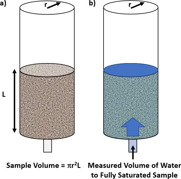
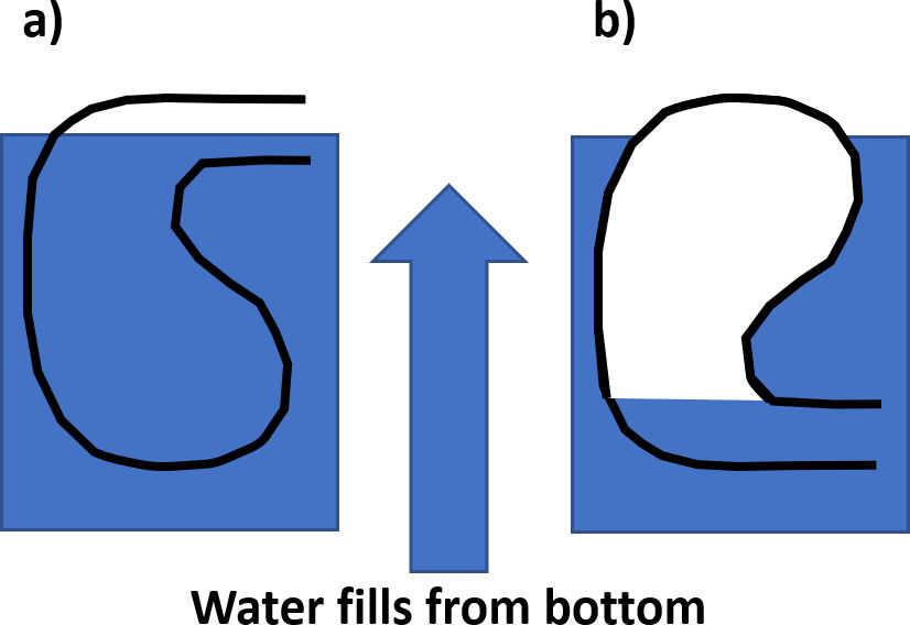
Effective porosity can be determined at the laboratory scale when sediment and rock samples of a given volume are dried and then the pore spaces are filled with water (Figure 8). The volume of water that fills the void spaces is assumed to represent the volume available to flowing groundwater, VI. For example, to determine the effective porosity of a granular earth material, a sample volume is collected, allowed to dry completely, and then water is introduced slowly to the base of the sample (so that air can escape from the top). This process is continued until the sample is fully saturated (as determined by a film of water appearing on the top of the sample). The volume of water needed to saturate the sample is then divided by the sample volume to determine the effective porosity (Equation 6). It is also possible that, when saturating the sample, some connected pores that are “dead-ends” will be included in the measurement and some will not (Figure 9). Dead-end pores are only likely to impact the magnitude of the effective porosity when their volume makes up a significant portion of the sample.
Effective porosity can also be determined by submerging a fully dried sample in a beaker filled with a measured quantity of water and applying suction to draw air out of the sample. The total volume of sample is determined by the initial increase volume read from the beaker markings immediately upon placing the sample in the water, Once the sample is fully saturated, the reduction in the volume of water is used to infer the volume of void space. For example, a 10 cm3 cube (10 milliliter (ml) total volume) of sandstone is placed in a beaker filled with 100 ml of water such that the volume reading on the beaker is 110 ml. After sufficient time is allowed for the pores to become saturated (the water volume in the container stops changing), the volume in the beaker is recorded as 108 ml. The volume of void space is 2 ml (2 cm3). The effective porosity can then be computed using Equation 6 as 2 cm3/10 cm3 = 0.20. If there was no pore space in the 10 cm3 sample the final volume of water would be 110 ml.
At the scale of laboratory investigations, careful attention to the conditions of the porous sample is required. Ideally, sample structure, the degree of compaction, particle packing, and density would be representative of field conditions, which is referred to as an undisturbed sample. However, in some cases, physical sampling methods may increase or decrease the sample porosity. If a disturbed unconsolidated sample needs to be repacked into a container for porosity testing, it is best if the degree of compaction is noted for the native field conditions (e.g., by using a cone penetrometer or a standard penetration test). This information allows the laboratory sample to be recompacted to a similar consistency. Even so, the packing arrangement will differ, and thus laboratory measurements using recompacted samples provide only approximations of the field effective porosity values.
Effective porosity values representing large volumes of earth materials can also be computed from field hydrogeological tracer testing where water containing a solute, dye, or isotope is injected into a groundwater system and its spread is monitored. Ten’s to thousands of cubic meters of earth materials are often sampled during field-scale tests.
Values of Effective Porosity
The effective porosity may equal, or be less than, the total porosity (n) of the sample (Table 1 and 2). In most cases, total porosity values reported for uncemented granular material and rocks with well‑connected pores and fractures can be used to represent effective porosity. Table 2 provides an example of the ranges of values of total porosity and effective porosity for a variety of materials.
Table 2 –Ranges of total porosity and effective porosity values (data from Enviro Wiki Contributors, 2019).
| Total and Effective Porosity | ||
| Total Porosity | Effective Porosity | |
| Unconsolidated Sediments | ||
| Gravel | 0.25 – 0.44 | 0.13 – 0.44 |
| Coarse Sand | 0.31 – 0.46 | 0.18 – 0.43 |
| Medium Sand | 0.16 – 0.46 | |
| Fine Sand | 0.25 – 0.53 | 0.01 – 0.46 |
| Silt, loess | 0.35 – 0.50 | 0.01 – 0.39 |
| Clay | 0.40 – 0.70 | 0.01 – 0.18 |
| Sedimentary and Crystalline Rocks | ||
| Karst and reef limestone | 0.05 – 0.50 | — |
| Limestone, dolomite | 0.00 – 0.20 | 0.01 – 0.24 |
| Sandstone | 0.05 – 0.30 | 0.10 – 0.30 |
| Siltstone | — | 0.21 – 0.41 |
| Basalt | 0.05 – 0.50 | — |
| Fractured crystalline rock | 0.00 – 0.10 | — |
| Weather granite | 0.34 – 0.57 | — |
| Unfractured crystalline rock | 0.00 – 0.05 | — |