8.1 Mapping the Head Distribution
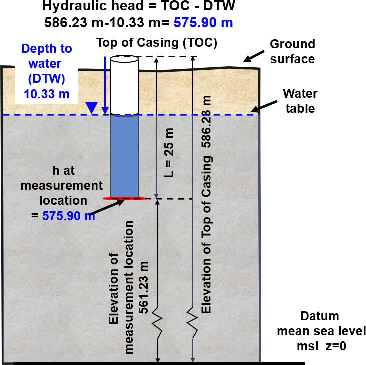
A plot of the spatial distribution of hydraulic head at a given time is used to interpret groundwater gradients, flow directions, fluxes and velocities. The elevation (relative to a horizontal datum, i.e., mean sea level) of the water level in a well bore represents hydraulic head. Head data are gathered in the field by surveying the location and elevation of the top of the casing (TOC) of wells or piezometers, then measuring from the top of the casing to the depth of the water level as shown in Figure 63. The depth to water is then subtracted from the TOC elevation to generate a head value (the elevation of the water level). Typically, a steel tape or an electric water-level-depth probe (dipmeter) is used to determine the depth to water. Wells can also be instrumented with electrical transducers that record the change in the depth of water overlying the transducer over a selected time interval.
It is recognized that measuring tools have errors associated with them. Neilson (1991) prepared a table comparing measuring methods and associated accuracy that showed instrument errors varied from 2 to 10 mm. Error also occurs during the survey of TOC elevations (survey error) and as a result of the approach the instrument operator uses to measure the water level (operator error). Thus, measured heads may have a combined error +/- that is larger than the instrument error. In most regional settings, values can be rounded to tenths of a meter to account for errors. When a small area is being evaluated or gradients are small, however, head differences of a few centimeters are usually needed to distinguish gradients and great care is required to minimize error during surveying and water level depth measurement. An error study that quantifies the measurement error associated with head values should be performed and results reported with raw head data and when discussing heads plotted on maps and cross sections.
The next step is to assign the head value to the correct position in a cross sectional or map view of the field site (Figure 64). The open portion of the well is the location of the head measurement. In Figure 63 it is at the bottom of the well. Some wells are perforated or screened over a portion of their length, this is called an open- or screened-interval. Such intervals may range from less than a meter to the entire well depth. In this case, the head value is typically plotted at the midpoint of the open interval. Once a number of head values are plotted on a cross section, the distribution of head (x,z) can be contoured creating equipotential lines. Equipotential lines connect locations of equal head (dashed red lines of Figure 64a). In map view, heads are plotted at the well casing locations (x,y) as shown in Figure 64b. The head values are independent of the surface elevation. Once a number of head values are plotted on a map, heads are then contoured creating equipotential lines and lateral flow directions are inferred.

The construction of cross sections and map views of head data is a standard practice. The map view for a confined or unconfined aquifer is referred to as a representation of the potentiometric surface. An example is shown for the confined Memphis Sand aquifer, Memphis, USA in Figure 65. A map of the total head for an unconfined aquifer can also be referred to as a water table map. However, because the water table is a representation of head (energy per unit weight) it is also referred to as representing a potentiometric surface. So, when using the term potentiometric surface, it should be placed in context as either representing a confined or unconfined groundwater system.
