5.5  Hydraulic Conductivity of Homogeneous and Heterogeneous Materials

William W. Woessner; Eileen P. Poeter

5.5 Hydraulic Conductivity of Homogeneous and Heterogeneous Materials

When hydrogeologic settings have homogeneous hydraulic conductivity distributions it is often the result of depositional process producing a fairly uniform set of conditions (e.g., conditions favorable to similar pore sizes and connections; similar sediment structures; followed by similar weathering and fracturing processes). From a geologic perspective, such conditions are most common in broad areas of sedimentation with similar processes (e.g., beach deposits, sand dunes, back bay deposits). Formations that were chemically precipitated (e.g., limestones, dolostones, salt) may initially be homogeneous. Post depositional processes such as dissolution, jointing, and fracturing may result in maintaining homogeneity or the development of heterogeneous conditions. Igneous and metamorphic rocks are initially relatively impermeable and may develop homogeneous or heterogeneous properties through a secondary process (e.g., weathering, solutioning, jointing, and fracturing). Certainly, some large scale, isotropic and homogeneous hydraulic conductivity conditions occur, but most unconsolidated and consolidated formations are anisotropic and heterogeneous. The primary cause of anisotropy on a small scale is the orientation of clay minerals in sedimentary rocks, unconsolidated layering in sediments, and fracture sets in crystalline materials. Core samples of clays and shales seldom show horizontal to vertical anisotropy greater than 10:1, and it is usually less than 3:1. However, at the field scale where coarse- and fine-grained materials are interlayered or fracture sets dominate, ratios of K_x to K_z can exceed 1000:1. In most hydrogeologic settings, heterogeneous and anisotropic distributions of hydraulic conductivity are the norm.

Equivalent Hydraulic Conductivity

Geologic formations often involve layered geologic materials in which each bed is isotropic and homogeneous. This is referred to layered heterogeneity. Sometimes the layers are thin and it is useful to obtain an equivalent representative hydraulic conductivity for a group of layers in order to make calculations such as determining flow rates or groundwater velocities through the material using Darcy’s law. An equivalent horizontal and vertical hydraulic conductivity can be derived for the layered unit.

A saturated two-layered system is represented in Figure 37. The layers are isotropic and homogeneous with different values of hydraulic conductivity, K₁ and K₂.

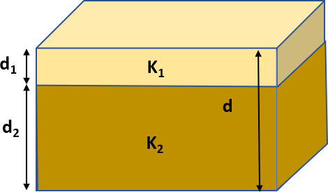
Figure showing two isotropic and homogeneous layers — **Figure 37 –** Two isotropic and homogeneous layers representing a geologic material with d = d₁ + d₂. The thickness of layer 1 is d₁ and the homogeneous, isotropic hydraulic conductivity is K₁. The thickness of layer 2 is d₂ and the homogeneous, isotropic hydraulic conductivity is K₂. In this example, K₁ > K₂.

The equivalent horizontal hydraulic conductivity, K_h, can be computed using a thickness-weighted arithmetic average as presented in Equation 36:

$\displaystyle K_h=\ \sum_{i=1}^{n}{\left[\frac{K_id_i}{d}\right]\ }$

(36)

and for conditions shown in Figure 37:

$\displaystyle K_h=\frac{K_1d_1+K_2d_2}{d_1+d_2}$

(37)

where:

K_h	=	equivalent horizontal hydraulic conductivity (L/T)
K₁	=	hydraulic conductivity of layer 1 (L/T)
K₂	=	hydraulic conductivity of layer 2 (L/T)
d	=	d₁ + d₂, total thickness (L)
d₁	=	thickness of layer 1 (L)
d₂	=	thickness of layer 2 (L)

An equivalent vertical hydraulic conductivity can be computed using a thickness-weighted harmonic average as presented in Equation 38:

$\displaystyle K_v=\ \frac{d}{\sum_{i=1}^{n}\frac{d_i}{K_i}}$

(38)

and for the two-layer condition shown in Figure 37:

$\displaystyle K_v=\frac{d_1+d_2}{\frac{d_1}{K_1}+\frac{d_2}{K_2}}$

(39)

For example, in Figure 37, if K₁ = 100 m/d and K₂ = 6 m/d, and d₁ = 10 m and d₂ = 30 m, the equivalent K_h would be 29.5 m/d (Equation 37). The equivalent K_v would be 7.8 m/d (Equation 39).

The theoretical basis for these expressions and an additional example of deriving equivalent hydraulic conductivities for a four-layer system is provided in Box 5. Click here to read Box 5.

There are likely as many types of heterogeneous configurations as there are geological environments, but it can be useful to draw attention to four broad classes described by Freeze and Cherry (1979): Layered heterogeneity, discontinuous heterogeneity, random heterogeneity and trending heterogeneity.

Layered heterogeneity is common in marine deposits, unconsolidated lacustrine deposits and sedimentary rocks. An example was described using Figure 37 and Equations 36 through 39. Layered heterogeneity can be comprised of materials with K values spanning nearly the full 13-order-of-magnitude range displayed in Figure 32, for example, in interlayered deposits of clay and sand.

Discontinuous heterogeneity can occur in the presence of large-scale stratigraphic features or faults that may have large contrasts in K (Figure 38). Another example of a discontinuous feature is the overburden-bedrock contact.

Figure showing discontinuous heterogeneity caused by faulting — **Figure 38 –** Discontinuous heterogeneity caused by faulting that juxtaposed formations of differing hydraulic conductivity.

Random heterogeneity can occur in the presence of a wide variety of geologic materials where mixtures of deposits that do not have any readily identifiable structure can be grouped as a unit for the purpose of calculating equivalent K values. If present, a non-random structure is often difficult to identify such as the K distribution shown in the units outlined by white in Figure 39. In this case, it has been found that calculating the geometric mean of the sample values produces and equivalent homogeneous isotropic value fairly representative of the unit as a whole (Equation 40).

Figure showing a cross-sectional view of five layers of volcanic rocks — **Figure 39 –** A cross-sectional view of five layers of volcanic rocks comprised of a mixture of materials with varying hydraulic conductivity values (dark colors represent low values and light colors represent high values of hydraulic conductivity). The individual formation hydraulic conductivity distributions within the white outlines do not have a readily identifiable structure. Equivalent hydraulic conductivities can be computed as the geometric mean of the sample values for each formation using Equation 40.

$\displaystyle K_{equivalent}={10}^{\left(\frac{1}{N}\sum_{i=1}^{i=N}\log{K_i}\right)}$

(40)

where:

K_equivalent	=	equivalent homogeneous isotropic value representative of the unit as a whole (L/T)
K_i	=	K for each of N samples from the unit (L/T)
N	=	number samples with measured K values (dimensionless)

Trending heterogeneity is illustrated on the map in Figure 40. Trends are possible in many types of geological formations, and are commonly observed in alluvial fans, deltas, and glacial outwash plains. Geologic facies representing sediments originating from different depositional environments are often mapped and can be used to identify trending heterogeneities. Variations in bedding, jointing and fracturing can also be linked to trending horizontal and vertical heterogeneity.

Figure showing trending heterogeneity — **Figure 40 –** Trending heterogeneity caused by a sedimentary process resulting from a geologic depositional environment with high energy in the southeast such that uniform coarse-grained materials were deposited in that area and declining energy to the northwest such that finer-grained sediments were deposited in that area.

The common heterogeneous conditions found in regional studies make assignments of equivalent hydraulic conductivity values difficult. Researchers have recognized that the hydraulic conductivity distribution in most formations follows a log normal distribution where the standard deviation of ln(K) can range from 0.5 to 4.5 (Meerschaert et al., 2013). Consequently, hydraulic conductivities derived from lab and field scale testing, are often correlated with knowledge of the geologic setting, published tables of values, as well as head and gradient information to generate representative hydraulic conductivity values. Estimates should be supported by field and laboratory measurements.

Equivalent Hydraulic Conductivity

License