6.4 Properties of Aquifers and Confining Units
The groundwater transmission and storage properties of geologic formations including aquifers and confining units can be described by three hydrogeologic terms: transmissivity, T; specific storage, Ss; and storativity, S.
Transmissivity
When describing the transmission capacity of a small representative volume of porous media the hydraulic conductivity is used. However, the capacity of an unconfined or confined aquifer to transmit water is described as transmissivity. Transmissivity is defined as the product of hydraulic conductivity, K, and saturated aquifer thickness, b, as shown in Equation 43.
| T = K b | (43) |
where:
| T | = | transmissivity, the capacity of an aquifer to transmit water (L2/T) |
| b | = | saturated thickness of the aquifer (L) |
The units of transmissivity are L2/T. The term transmissibility is an outdated term that is occasionally used for transmissivity. Transmissivity describes the overall transmission capacity of an aquifer system, not just the properties of a small volume of the aquifer. For example, if the hydraulic conductivity of a confined aquifer is 100 m/d and the thickness is 10 m, then T is 1,000 m2/d. If another aquifer has a hydraulic conductivity of 50 m/d and is 300 m thick, its transmissivity is T = 15,000 m2/d. The higher T of the second aquifer indicates that it can transmit more water, thus if all else is equal, it would be a better target for a water supply well. Aquifers with multiple horizontal layers with different hydraulic conductivities can be represented by the sum of the T value for each layer.
The transmissivity of a confined aquifer of uniform thickness is a constant value for an isotropic and homogeneous set of conditions as shown in Figure 48a. By definition the head of a confined aquifer is higher than the top of the aquifer, so the complete thickness of the confined aquifer is saturated, thus b is a constant when T is determined. The saturated thickness of an unconfined aquifer varies with space as the water table slopes in the direction of flow, thus, T values change with distance from a given location (Figure 48b). When the water table slope is small, a single value of T is commonly used to represent the aquifer. In areas with large water table gradients, average thickness may be used to compute one representative value of T.

Transmissivity values are often estimated by combining K values from laboratory tests or textbook tables with field measurements of aquifer thickness, b. Most commonly, T values are determined from carefully designed aquifer tests were wells are pumped while water levels are measured in nearby observation wells. These data are then analyzed using analytical equations and/or numerical computer simulations to estimate transmissivity values (e.g., Lohman, 1972).
Storativity
The storage capacity of an aquifer is referred to as the storativity, S. The older term, storage coefficient, is also used to describe the same aquifer storage property. Storativity describes the capacity of an aquifer to store or release water. It is defined as the volume of water removed or stored per unit change in head normal to the earth’s surface over a unit area. Storativity is dimensionless and is expressed as a decimal.
Unconfined Aquifer Storativity
The storativity for an unconfined aquifer is dominated by the gravity drainage term, specific yield (Sy). Specific yield reflects the volume of water that drains by gravity when the water table is lowered, or fills with water when the water table is raised (Figure 49). The storativity (S) of an unconfined aquifer is composed of two components as shown in Equation 44.
| Sunconfined = Sy + Ssbaverage | (44) |
where:
| Sunconfined | = | storativity of an unconfined aquifer (dimensionless) |
| Sy | = | specific yield (dimensionless) |
| Ss | = | specific storage (1/L) |
| baverage | = | average thickness before and after a water level change (L) |

The specific yield is the volume of water that can drain by gravity from a saturated volume of material divided by the total volume of that material. The fractional volume of water that remains in the sample is called specific retention (Sr). It is assumed that, when water is added to storage and the water table rises, the pore spaces that fill already contain only the volume of water indicated by the value of specific retention.
The second term of Equation 44 is the product of the specific storage (Ss) and the average of saturated thickness before and after drainage (baverage). The specific storage is defined as the volume of water that is released from (or added to) storage per unit volume of saturated material. When multiplied by the saturated thickness it accounts for a small amount of water that is released from a unit area of aquifer in response to the relief of stress on the material below the drained pores. When the head declines the water that is released from saturated storage through the column of aquifer underlying drained pores is produced by two mechanisms: (1) the compaction of the aquifer (reduction in pore volume) caused by an increase in the effective stress, σe, and (2) the expansion of the water caused by decreased pore water pressure. Effective stress is the difference between the total pressure exerted by the overlying material (soil/rock and water combined) minus the pore water pressure. An increase in pore water pressure lifts the grains of the aquifer skeleton thus relieving the stress of the overlying material on the grains. The first of the mechanisms that releases water from an aquifer for a head decline is controlled by the aquifer compressibility, α, and the second by the fluid compressibility, β. The volume of water in the porous medium is dependent on the effective porosity, ne. The resulting equation for Ss is Equation 45.
| Ss = ρg (α + neβ) | (45) |
where:
| Ss | = | specific storage (1/L) |
| α | = | compressibility of the aquifer solid structure (T2L/M) |
| ne | = | effective porosity (dimensionless) |
| β | = | compressibility of water (T2L/M) |
To account for the thickness of saturated media that is affected by the change in pore water pressure and the consolidation of the aquifer skeleton, the specific storage is multiplied by the average saturated thickness for the given water table decline, baverage (Figure 49), resulting in a dimensionless storativity term as shown in Equation 46.
| Sunconfined = Sy + Ssbaverage = Sy + baverageρg (α + neβ) | (46) |
where:
| Sunconfined | = | Storativity of an unconfined aquifer (dimensionless) |
The compressibility of water is small, 4.4 × 10⁻¹⁰ m2/N (N is a Newton = 1 (kg m)/s2) and the compressibility of earth materials ranges from 1 × 10-11 to 1 × 10⁻⁶ m2/N (Table 4). The scale of the Ssbaverage term is illustrated with this example. For an unconfined sand aquifer with a compressibility on the higher end of the range, α = 1 × 10⁻⁸ m2/N, an effective porosity of 0.24, a water density of 1 kg/m3 and with g = 9.8 m/s2, then the specific storage (Equation 45) is 1 × 10⁻⁷/m. If the aquifer is 60 m thick then the storage term related to the remaining saturated aquifer (Equation 46) is 6 × 10⁻⁶. The computed Ssbaverage value is more than three orders of magnitude smaller than the Sy, given typical specific yields of earth materials range from 0.05 to 0.40, so the storativity term for the unconfined aquifer can be set equal to Sy and the Ssbaverage term can be ignored as presented in Equation 47.
| simplified Sunconfined = Sy | (47) |
In fact, when Sy is obtained by a field test involving pumping a well and observing the changing water levels in nearby observation wells, the volume of water from Ssbaverage is “built in” to the interpreted Sy value (e.g., Lohman, 1972). Equation 47 is typically used to represent specific yield.
Table 4 Range of values of compressibility of earth materials and water (after Domenico and Mifflin,1965; Freeze and Cherry, 1979).
| Compressibility of Some Common Earth Materials | |
| Material | Compressibility (meter2/Newton) |
| Geologic Type | Range of Compressibility α |
| Clay | 1 × 10⁻⁶ – 1 × 10⁻⁸ |
| Sand | 1 × 10⁻⁷ – 1 × 10⁻⁹ |
| Gravel | 1 × 10⁻⁸ – 1 × 10⁻¹⁰ |
| Jointed Rock | 1 × 10⁻⁸ – 1 × 10⁻¹⁰ |
| Sound Rock | 1 × 10⁻⁹ – 1 × 10-11 |
| Fluid | Compressibility β |
| water | 4.4 × 10⁻¹⁰ |
The volume of water removed from or added to aquifer storage over an area, A, for a change in head, ∆h, is determined as shown in Equation 48. For a specific yield of 0.18, if the water table declined 1 meter over a 1 square meter area, then 0.18 cubic meters would drain from the aquifer. If the area were instead 1 km2, then 180,000 cubic meters would drain from the aquifer.
| Volume of Unconfined Water for a change in head = SyA∆h | (48) |
where:
| Volume | = | volume drained from an unconfined aquifer over an area, A, for a water table elevation change of ∆h (L3) |
| Sy | = | specific yield (dimensionless) |
| A | = | area over which the water table changes (L2) |
| ∆h | = | change in water table elevation (L) |
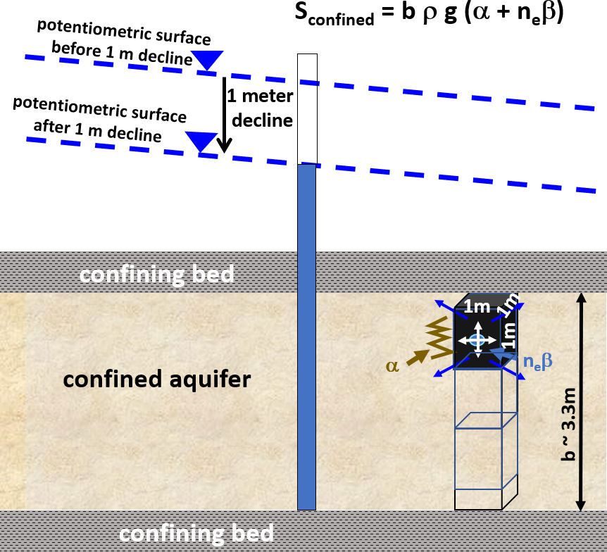
Confined Aquifer Storativity
The storativity of a confined aquifer is defined as the volume of water released from, or added to, storage per unit change in head normal to the surface, per unit area. This is the same definition as for unconfined aquifers. The difference between the storage capacity in an unconfined aquifer and a confined aquifer is that in the confined aquifer the entire aquifer remains saturated when a unit change in head occurs (Figure 50). As a result, no gravity drainage occurs and all the water that leaves or enters storage is derived from the specific storage term, Ss, times the saturated thickness, b, as shown in Equation 49.
| Sconfined = Ssb = bρg (α + neβ) | (49) |
where:
| Sconfined | = | storativity of a confined aquifer (dimensionless) |
The specific storage of a confined aquifer can be computed as described Equation 45, with Sy = 0. This value is then multiplied by aquifer thickness to obtain storativity (Equation 49). Storativity of confined aquifers typically range from 0.00001 to 0.001 (1 × 10⁻⁵ to 1 × 10⁻³). Lohman (1972) suggests the storativity for a confined aquifer can be approximated as 0.0000033/m (0.000001/ft) times the aquifer thickness in meters. Most commonly, site and regional scale confined aquifer storativity values are derived from carefully designed aquifer tests where the aquifer is pumped for a period of time and the response the total head distribution monitored (e.g., Lohman, 1972).
The volume of water removed from or stored in a confined aquifer over an area, A, for a change in head, Δh, is determined as shown in Equation 50. For a storativity of 0.00001, if the water table declined 1 meter over a 1 square meter area, then 0.00001 cubic meters would be released from the aquifer. If the area were instead 1 km2, then 10 cubic meters would be released from the aquifer. The volume of water released from a confined aquifer for a given head decline is substantially less than the volume released from an unconfined aquifer for the same head decline. This is because the water comes only from the compression of the aquifer framework and expansion of water in response to the pressure change rather than from drainage of pore spaces.
| Volume of Confined Water for a change in head = SAΔh | (50) |
where:
| Volume | = | volume drained from a confined aquifer for a hydraulic head change, Δh, over an area, A (L3) |
| S | = | storativity (dimensionless) |
| A | = | area over which the head change occurs (L2) |
| Δh | = | change in head (L) |