Box 5 Equation Derivation for Equivalent K and a 4-layer Application
To calculate the equivalent hydraulic conductivity parallel to layers, Kx, consider flow through the system shown in Figure Box 5-1. Define ∆h as the hydraulic head difference over a horizontal distance ΔLx (so that ∆h/ΔLx is the hydraulic gradient). The volumetric discharge Q (L3/T) through a unit width (into the image) of the system is the sum of the volumetric discharges through each layer. The specific discharge is q = Q/A. Here the area is equal to the product of the thickness d and one unit of distance into the image, so A=d(1), thus q = Q/d(1), or q = Q/d. Knowing that q = −Ki, this logic can be applied to the stack of layers as follows in Equations Box 5-1 through Equation Box 5-3. Equation Box 5-1 indicates the horizontal flow through each layer.

 |
(Box 5-1) |
where:
| Qi | = | volumetric discharge through an individual layer of a unit width denoted by i (L3/T) |
| di | = | thickness of individual layer i (L) |
| ΔLx | = | length of the layers in the x-direction (L) |
| ∆h | = | hydraulic head difference over horizontal distance ΔLx (L) |
Equation Box 5-2 provides the specific discharge for the entire section by summing the flow through every layer and dividing by the total flow area of the section, and shows that the specific discharge for the entire stack of layers is equal to the product of the equivalent Kx and the gradient.
![\displaystyle q=-\sum_{i=1}^{n}\left [ \frac{K_{i}d_{i}}{d} \right ]\frac{\Delta h}{\Delta L_{x}}=-K_{x}\frac{\Delta h}{\Delta L_{x}}](https://books.gw-project.org/hydrogeologic-properties-of-earth-materials-and-principles-of-groundwater-flow/wp-content/ql-cache/quicklatex.com-3b02a7b5a24f4b2ff8c7136c30ad9568_l3.png "Rendered by QuickLaTeX.com") |
(Box 5-2) |
where:
| q | = | specific discharge through the entire section per unit width in the horizontal direction (L) |
| Kx | = | equivalent Kx of the entire section (L/T) |
Then, simplifying Equation Box 5-2 by cancelling the gradients, the equivalent K in the x direction is as shown in Equation Box 5-3.
![\displaystyle K_{x}=\sum_{i=1}^{n}\left [ \frac{K_{i}d_{i}}{d} \right ]](https://books.gw-project.org/hydrogeologic-properties-of-earth-materials-and-principles-of-groundwater-flow/wp-content/ql-cache/quicklatex.com-2836e209f992276ca7323ee63cf140ea_l3.png "Rendered by QuickLaTeX.com") |
(Box 5-3) |
This calculation of the equivalent Kx for the layered formation is a thickness-weighted arithmetic mean. This is the same as Kh, equivalent horizontal hydraulic conductivity, referred to in the main text. Some readers may find it useful to note that the equation for calculating equivalent K parallel to layers is identical to the equation used to calculate the equivalent conductance through electrical resistors that are wired in parallel.
To calculate the equivalent the hydraulic conductivity perpendicular to the layers, Kz, consider vertical flow through the system shown in Figure Box 5-2. Let ∆h be the hydraulic head difference over a vertical distance ΔLz (so that, ∆h/ΔLz is the overall hydraulic gradient). Mass must be conserved, so the volumetric inflow Q (L3/T) through a unit width (into the image) of the system at the bottom must be equal to the outflow at the top. In fact, water cannot be created nor destroyed along the flow path, so the specific discharge must be the same through each layer of the system. Given that the hydraulic conductivities differ between layers, then by Darcy’s law, with a constant flow rate through each layer, the gradient will be different in each layer, as indicated by Equation Box 5-4.
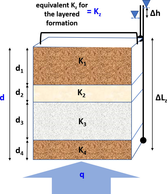
 = =  = =  = =  = =  |
(Box 5-4) |
where:
| q | = | specific discharge in the vertical direction (L/T) |
| ∆hi | = | hydraulic head difference across each layer in the vertical direction, the values of ∆hi sum to ∆h (L) |
| Kz | = | equivalent Kz of the entire section (L/T) |
Rearranging Equation Box 5-4 produces Equation Box 5-5, where ∆h is expanded into the sum of the layer ∆hi values, and, by Darcy’s law, each ∆hi can be expressed as qdi / Ki.
 = =  = =  |
(Box 5-5) |
By cancelling the q’s and summing the dz / Ki, Equation Box 5-6 provides the procedure for calculating the equivalent Kz.
 |
(Box 5-6) |
This calculation of the equivalent Kz for the layered formation is a thickness-weighted harmonic mean. It is the same value as the Kv, equivalent vertical hydraulic conductivity in the main text. Some readers may find it useful to note that the equation for calculating equivalent K perpendicular to layers is identical to the equation used to calculate conductance through electrical resistors that are wired in series.
Equations Box 5-3 and Box 5-6 provide the Kx and Kz values for a homogeneous but anisotropic formation that is hydraulically equivalent to the layered heterogeneous system of homogeneous, isotropic geologic formations (Figure Box 5-3). Given that Kx is a thickness-weighted arithmetic mean, the high hydraulic conductivity values dominate its value, whereas the low hydraulic conductivity layers dominate the thickness-weighted harmonic mean Kz value. For example, suppose the materials from top to bottom are coarse sand, medium gravel, silty sand and fine gravel. The layers from top to bottom have K values of K1 = 100 m/d, K2 = 1000 m/d K3 = 0.1 m/d and K4 = 400 m/d and corresponding thicknesses of d1 = 125 m, d2 = 58m, d3 = 125 m and d4 = 67 m. The computed horizontal and vertical hydraulic conductivities are Kx = 260 m/d and Kz = 0.3 m/d (using Equations Box 5-3 and Box 5-6). The anisotropy ratio, Kx/Kz, is on the order of 900. In the field, it is common for layered heterogeneity to lead to regional anisotropy values on the order of 10:1 and in many settings much greater values.
