8.3 The Influence of Boundary Conditions
Generally, groundwater system boundaries can be referred to as physical boundaries or hydraulic boundaries. Physical boundaries do not move as the flow directions and rates within a groundwater system change. They represent a measurable change in hydrogeologic properties such as those that occur at formation contacts, faults, and large water bodies. Hydraulic boundaries can move when the flow field changes because they are formed by hydraulic conditions such as locations and rates of recharge and the divergence or convergence of multiple flow systems.
Physical Boundaries
Non-flow or Zero Flux Boundaries
Physical boundaries such as a hydraulic conductivity contrast, control flow paths in a groundwater system. For example, if a permeable sand and gravel aquifer abuts a low hydraulic conductivity granite, the groundwater flow within the aquifer parallels the boundary (Figure 72a) and the equipotential lines meet the boundary at right angles (Figure 72a). This is a Type 2 specified flux boundary referred to as a no-flow or zero flux boundary.
Constant Head Boundaries
In contrast, if a large lake forms a boundary of the aquifer, groundwater flow lines are perpendicular to the lake shore because the water level of the lake is an equipotential line, so equipotential lines in the aquifer near the lake are parallel to the boundary (Figure 72b). This boundary is a specified head Type 1 boundary, referred to as a constant head boundary.
Water Table Boundary
The water table is the upper boundary of an unconfined aquifer. A water table is a unique boundary in that pressure head is, by definition, zero so head is equal to elevation. If recharge enters the unconfined aquifer, water flows across the boundary at an angle and equipotential lines meet the water table at an angle (Figure 72c). If there is no recharge, the water table is a flow line the equipotential lines meet the water table at right angles (Figure 72d). Regardless of whether flow occurs across the water table, or not, the value of an equipotential line where it intersects the water table is equal to the elevation of the water table.

Boundaries at Subsurface Features
Faults
Faults or shear zones can also form physical flow boundaries (Figure 73). The behavior of groundwater in the vicinity of these features depends on whether the faulting created conditions that significantly reduced the hydraulic conductivity (e.g., by creating fault gouge, or juxtaposing formations of substantially different hydraulic conductivity) or enhanced the hydraulic conductivity (e.g., by creating numerous, well-connected, open, large aperture fractures within and adjacent to the feature). When fault or shear zones restrict groundwater flow, they may be considered Type 2 no-flow boundaries. If a conductive fault zone is located near the perimeter of the model domain and is connected to a source of water, it may be treated as a Type 2 constant flux or Type 3 variable flux boundary. In some settings, conditions within a single zone vary spatially such that some sections may enhance flow while others limit flow. It is advisable to inspect outcrops and place wells near and within faults and shear zones to determine if they limit or enhance flow.

Seawater-Freshwater Interface Boundaries
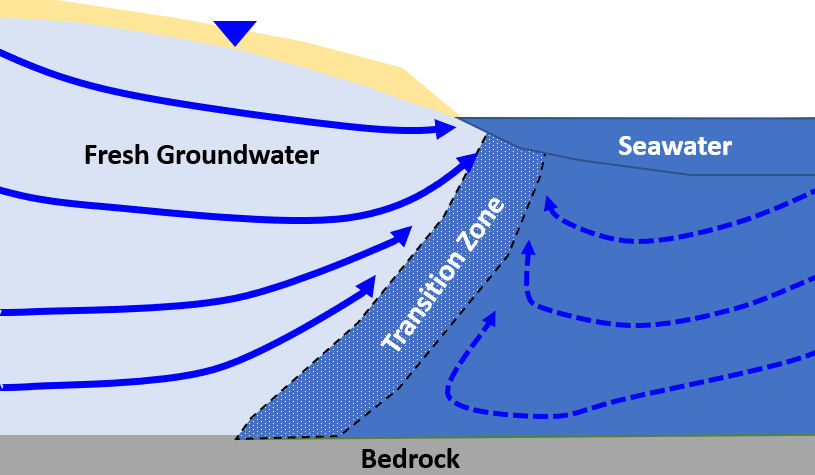
Near coastlines the subsurface seawater-groundwater interface creates a boundary to fresh groundwater flow (Figure 62 and Figure 74). The boundary acts as a physical boundary that limits flow, forcing fresh unconfined groundwater to discharge along the coastline. The interface behaves as a Type 2 no-flow boundary. The boundary is not a sharp interface because its position shifts with the tidal cycles and as freshwater discharge rates vary. A mixing zone between freshwater and seawater occurs and is referred to as the transition zone. Groundwater flow projects near coastlines often require modeling tools that account for variable density flow. In its simplest form it can be assumed the boundary acts as an impermeable physical boundary.
Hydraulic Boundaries
Hydraulic boundaries form when two or more flow systems converge. They are defined where parallel groundwater flowlines separate groundwater flows originating from common or differing recharge sources. They are typically drawn on cross sections, but sometimes hydraulic divides at recharge and discharge areas are indicated on maps. Hydraulic boundaries occur in both unconfined and confined systems.
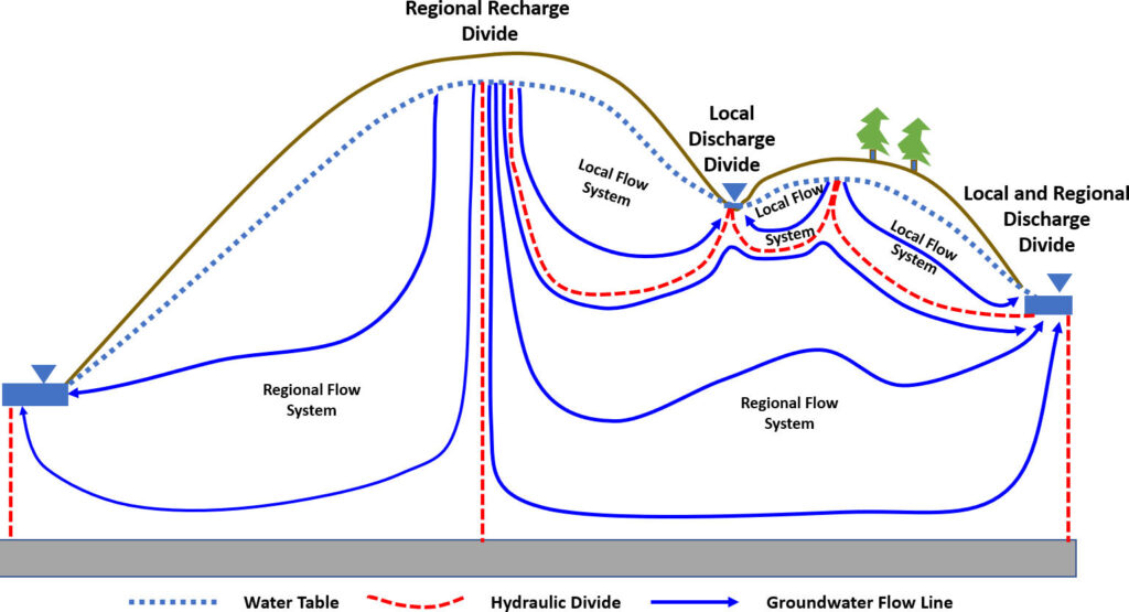
In an unconfined system, groundwater flow lines originate in a recharge area and continue to discharge areas. A vertical hydraulic divide is formed below both the recharge area and the discharge area (Figure 75, red dashed lines). As groundwater flow paths cannot cross, the divide boundaries act as no flow boundaries (Type 2). When a drop of water recharges the system on the divide, half of the drop moves along one side of the divide and the other half along the other side. Divides can be vertical, horizontal or some combination of conditions depending on the nature of the flow systems (Figure 75). Hydraulic boundaries are defined by the flow system conditions. They can change with time, including, in some cases, disappear as the head distribution changes in response to variations in the magnitude and timing of recharge and discharge.
Flow Systems with Distant Boundaries
It is not unusual to assess groundwater flow conditions in a portion of the system that is a long distance from physical boundaries. This problem domain would be considered to have distant boundaries. In some cases when analytical solutions are developed it is assumed that the boundaries impacting groundwater flow are sufficiently distant that the aquifer can be thought of as infinite in extent, a factor that simplifies the mathematics.
When groundwater modeling techniques are used and physical boundaries of the domain area are far away from a site of investigation, setting up local boundaries for the investigation may be appropriate. As an example, examine the setting shown in Figure 76a. Assume the area of interest is shown by the concentration of wells near the lake. The sand and gravel aquifer is unconfined, assumed to behave as an isotropic and homogeneous system, and is surrounded by a number of physical boundaries. These physical boundaries include a fault and low permeable granites to the south, water flowing out of the Green Mountains on the west, a major river to the north, and the lakeshore to the east. The purpose of the investigation is to determine the effect of pumping a new well (the location shown by the orange dot) on the water levels in existing wells in the area. In this setting, it may be appropriate to set local boundaries in the vicinity of the site of interest (Figure 76b). The lake elevation (a physical boundary of constant head (Type 1)) is set to the east. The western boundary is designated as a constant head (Type 1) using the value of the equipotential line established from contouring head measurements. The northern and southern boundaries are designated as no-flow (Type 2) because they are parallel to defined groundwater flow lines. This smaller model area is appropriate under transient flow conditions when the area of influence of the well (red dotted line in Figure 76b) is small and not affected by the local boundary conditions on the north, west, and south (impacting the eastern boundary would not be a problem because it is a physical boundary). However, if the area of influence is large like that shown in Figure 76c then the selection of the smaller area would not be appropriate because the artificial boundaries will influence the results. It should be noted that, if steady-state pumping was being investigated the local boundaries would influence the predictions. Steady-state analyses should be performed using the entire problem domain.
