
5.3 Storage Parameters
Confined Aquifers—A Conceptual Understanding
Let’s consider a confined aquifer that consists of a layer of sand overlain by a layer of clay that acts as a confining layer. If we install a well into the aquifer and pump water out of it, the water level in the well will decline. This reduction in water level caused by pumping is called drawdown. As pumping continues the water levels in the aquifer around the well also begin to decline in a way that results in the formation of a cone of depression in the potentiometric surface (Figure 24). The more we pump from the well, the larger the depth and areal extent of the cone of depression. The example in Figure 24 shows that a volume of water has been removed from the aquifer—reflected by the volume in the barrel—and has lowered the water level in the well and in the surrounding aquifer. However, we have not changed the saturated thickness of the aquifer itself—that is, the aquifer is still saturated up to the base of the confining layer. What is the source of the water in the barrel—that is, where does that water come from if all the pore space in the aquifer is full? It is released as the aquifer framework compresses and the sand grains and water in the aquifer pores expand slightly.
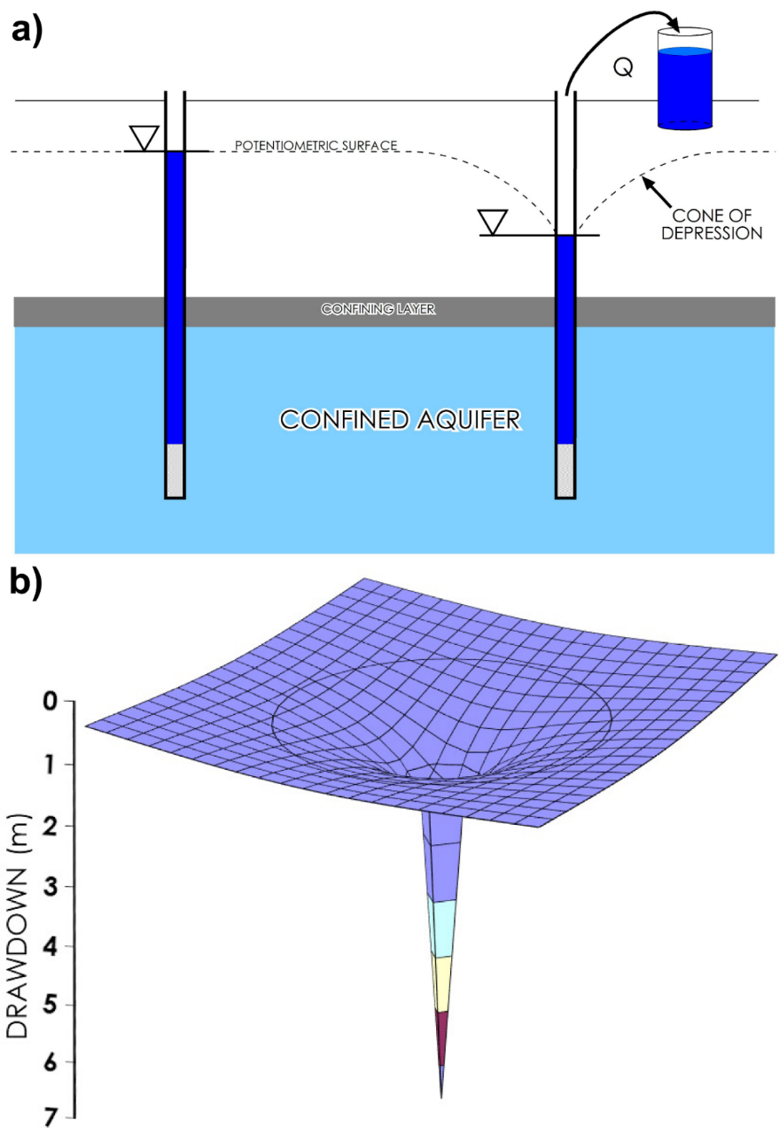
Figure 24 ‑ a) Changes in the potentiometric surface in response to pumping from a well in a confined aquifer; b) 3‑D view of a typical cone of depression centered around a pumping well.
An unconfined aquifer is made up of rock or sediments with pore spaces that are full of water. When there is no confining layer and the aquifer is recharged by water infiltrating from above, the pore spaces are full of water and the pore fluid pressure at any depth in the aquifer is equal to atmospheric pressure plus the pressure created by the weight of the overlying column of water. Therefore, in an unconfined aquifer, you can fit a volume of water into the pore space that is equal to the volume of the pore space.
However, if the aquifer is confined and an additional component of pressure is added to the water (as shown in Figure 25), the additional pressure will effectively force a greater volume of water into the pores of the sand. It does this by pushing the sand grains around so that pore volume is increased, and slightly compressing the water and the sand grains. This increased pressure and volume causes water levels in the aquifer to rise above the top of the aquifer—unlike an unconfined aquifer in which the water level defines the top of the aquifer. Increasing the pore fluid pressure causes the aquifer to undergo elastic deformation—that is, the change in volume is recoverable—so that a subsequent decrease in fluid pressure will cause an associated decrease in overall deformation of the pore spaces as illustrated in Figure 25.
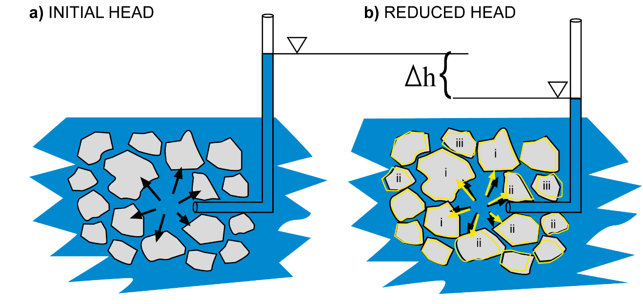
Figure 25 – Schematic of elastic deformation in a confined sand aquifer related to changes in fluid pressure. Gray polygons represent grains of sand, blue represents saturated pores between the sand grains, black arrows and the height of the blue column represent the fluid pressure in the large pore in the middle of the diagram. a) High pressure head pushes grains of sand apart (greatly exaggerated in this image), compresses water molecules by a small but measurable amount, and compresses individual sand grains by a nearly imperceptible amount. b) When head decreases, pressure is lower and sand grains move closer together, water molecules expand slightly, and sand grains expand a nearly imperceptible amount. The yellow grain outlines in (b) show the original sizes and locations of the sand grains as depicted in (a). The yellow arrows in (b) show the magnitude of pressure in (a). The lowercase letters in (b) represent examples of changes due to the reduction in fluid pressure: i = individual grain size increase, ii = sand grains that moved closer together, and iii = sand grains that rotated to accommodate reduced pore space.
The tiny changes in pore volume associated with movement and rotation of sand grains is the source of the volume of water that is removed from a confined aquifer. Pumping water from the confined aquifer lowers the fluid pressure—that is, the pressure head above the top of the aquifer—causing the aquifer to ‘relax’ and yield water that is stored by the excess pressure.
Confined Aquifers—A Mathematical Understanding
Now that we have a basic conceptual understanding of elastic storage of water in a confined aquifer, let’s describe this concept mathematically. What we as hydrogeologists are interested in knowing is what volume of water is associated with a given decline in head in the aquifer, or conversely, how much head loss will be associated with a given volume withdrawn from an aquifer.
Let’s consider a unit volume of our confined aquifer—by unit volume we mean a cube with some convenient dimensions like 1 meter cubed. This unit volume is saturated with water, and the water has an additional component of pressure that causes the water to rise above the top of the cube (Figure 26). If we remove some volume of water from the cube, we will reduce the additional component of pressure and lower the head in the cube. Removing more water will cause more head loss; less water will cause less head loss. Therefore, by trial-and-error we can determine the volume of water that needs to be removed to cause a unit decline in head—in this case, a head decline of one meter.
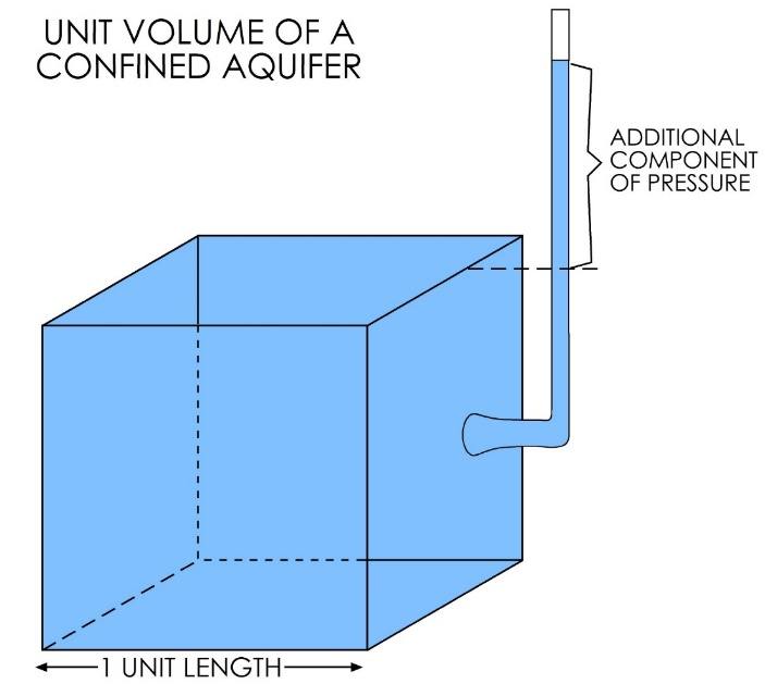
Figure 26 ‑ Unit volume of a confined aquifer.
This number that we measure—the volume of water per unit volume of aquifer that results in a unit decline in head—is the specific storage, given as [latex]S_{s}[/latex] in the groundwater flow equation. The specific storage is an aquifer storage parameter that mathematically describes the volume of water that can be withdrawn from a unit volume of a confined aquifer for a unit decline in head. This value is also called the elastic storage coefficient, as it deals only with the amount of water removed from elastic storage as described in the previous section and depicted in Figure 25. The specific storage is a function of the compressibility of the aquifer matrix—in this case, the sand—and the compressibility of water. It is rigorously defined as shown by Equation (40).
| [latex]S_{s} = \rho_{w}g\varphi(\alpha + \beta)[/latex] | (40) |
|---|
where (parameter dimensions are dark green font with mass as M, length as L, time as T):
| [latex]\rho_{w}[/latex] | = | density of water (ML-3) |
|---|---|---|
| [latex]g[/latex] | = | gravitational acceleration (LT-2) |
| φ | = | porosity (:) |
| α | = | compressibility of the aquifer matrix (LT-2M-1) |
| β | = | compressibility of water (LT-2M-1) |
Because we are dealing with a unit volume of aquifer and a unit decline in head, the specific storage refers to a point in the aquifer. However, when we are dealing with aquifers in a field setting, the thickness of the aquifer has an influence on how much water the aquifer will yield; given the same aquifer material, hydraulic conductivity, and porosity, a thicker aquifer will transmit and yield more water than a thinner aquifer. If we multiply the hydraulic conductivity of the aquifer by the aquifer thickness, we get a quantity called the transmissivity ([latex]T[/latex]), which describes the amount of water that can move through a unit width of the fully saturated thickness of the aquifer under a hydraulic gradient of one. Similarly, we have a quantity called the storativity ([latex]S[/latex]), which for a confined aquifer is the specific storage multiplied by the saturated thickness of the aquifer, as shown in Equation (41).
| [latex]S = S_{s}b[/latex] | (41) |
|---|
where (parameter dimensions are dark green font with mass as M, length as L, time as T):
| [latex]b[/latex] | = | saturated thickness of the aquifer (L) |
|---|
In other words, the storativity describes the volume of water removed from a unit area of aquifer for a unit decline in head.
Thought Question 6: Use dimensional analysis to determine the dimensions (or the units) of specific storage and of storativity.
A more detailed discussion of the theory behind confined aquifer storage parameters can be found in Groundwater Storage in Confined Aquifers↗ by Wang (2020) which is available from The Groundwater Project as a free download or can be read online.
Unconfined Aquifers
In a confined aquifer, all the water pumped out via a well is provided by the release of water in elastic storage. In an unconfined aquifer, we see the same thing—the changes in head result in a release of a small amount of water from elastic storage in the aquifer. However, as the water level declines, we also remove water from pore spaces as the water table declines which dewaters a section of the aquifer (Figure 27). This drainage of the aquifer’s pores produces a greater volume of water for an equal decline of head as compared to a confined aquifer.
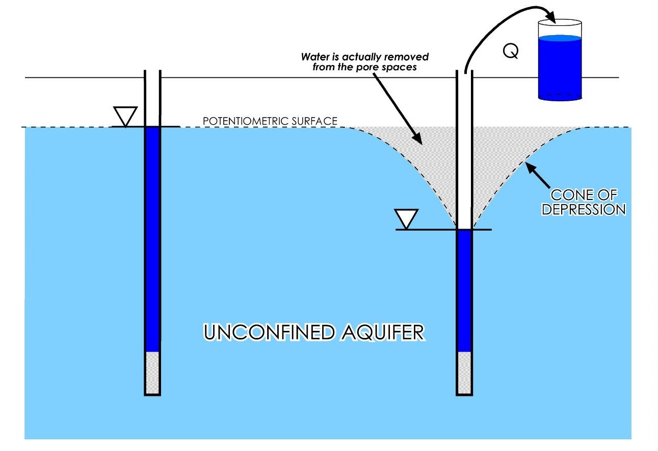
Figure 27 ‑ Changes in the potentiometric surface (i.e., water table) in response to pumping from a well in an unconfined aquifer.
This additional volume of water that drains from the pore spaces is characterized by a parameter called specific yield. As described in Section 3.2.3, specific yield is the volume of water that drains from a rock under the force of gravity and is essentially equivalent to the effective porosity of the aquifer matrix. The volume of water released from a unit volume of aquifer due to dewatering of the aquifer is therefore just the unit volume times the specific yield. For example, a 1 cubic meter volume of aquifer with a specific yield of 0.1 will yield 0.1 cubic meters of water for each 1‑meter decline in hydraulic head.
In unconfined aquifers, therefore, the volume of water released from a unit volume of aquifer is a function of both the specific yield—that is, the water removed from the pore space—and the specific storage—the water released from elastic storage in the aquifer. Therefore, in an unconfined aquifer, the storativity of the aquifer is the sum of the specific yield and the thickness times the specific storage, as shown in Equation (42).
| [latex]S = S_{y} + S_{s}\ b[/latex] | (42) |
|---|
The magnitudes of these parameters, however, are drastically different: Specific yield (i.e., effective porosity) values in an aquifer generally range from 1 percent to 50 percent, or 0.01 to 0.5, while specific storage values generally range from 1×10‑6 to 1×10‑4 m-1 or 0.000001 to 0.0001 m-1. This means that, in an unconfined aquifer, the volume of water provided by release from elastic storage is orders of magnitude less than that provided by dewatering the pores, so we generally assume that the specific storage is negligible and such that unconfined storativity as only the specific yield. In fact, when aquifer are tested the value obtained for specific yield incorporates what is yielded from elastic storage.
Thought Question 7: Consider two aquifers; each has the same porosity, permeability, and saturated thickness, but one is confined while the other is unconfined. If identical wells are installed in each and pumped at the same rate for the same period of time, in which aquifer would you expect to observe greater drawdown? Why?