
8.4 Aquifer Test Analysis
The following is a general, simplified discussion of the analysis of aquifer test data. A detailed and comprehensive overview of aquifer testing procedures and data analysis methods is provided in An Introduction to Hydraulic Testing in Hydrogeology: Basic Pumping, Slug, and Packer Methods↗ by Woessner and others (2020), which is available as a free download from The Groundwater Project. Professionals and students who are interested in aquifer testing are encouraged to download and review that book.
The Theis Curve‑Matching Method for Non‑Leaky (i.e., fully confined) Aquifers
The data set produced by a multi‑well aquifer test with a single observation well includes a pumping rate, a distance from the pumping well to the observation well, and a set of time‑drawdown data—that is, values for drawdown at various times after the start of pumping. Analyzing the data using the traditional Theis curve‑matching method requires the following steps.
- Obtain a Theis equilibrium type curve graph and a blank log‑log graph that has the same scale as the Theis type curve. A blank log‑log graph is provided as Figure 43 and the type curve with the same scale is provided as Figure 44.
- Plot the time‑drawdown data on the blank log‑log graph. An example is shown in Figure 45a.
- Overlay the time‑drawdown data graph on the type curve—it is best to use a light table or tape the type curve on a window or white computer screen—and move the graph until the data line up with the type curve. It is essential that the axes on both graphs are parallel during the matching procedure; otherwise, the match will not be correct. An example is shown in Figure 46a
- Select a corresponding point on each graph and determine the values of u and W(u) for that point on the time‑drawdown graph. The point does not have to fall on the Theis curve; it only needs to be in an area where both graphs overlap so a common match point can be determined. An example is provided in Figure 46b.
- Re‑arrange the Theis equation—Equation (73)—to solve for [latex]T[/latex] and substitute the values of [latex]s[/latex]and [latex]W(u)[/latex] from the curve match point to determine [latex]T[/latex]. The re‑arranged equation is shown as Equation (76).
| [latex]T = \frac{Q}{4\pi s}W(u)[/latex] | (76) |
|---|
- Re‑arrange the equation for [latex]u[/latex] shown as Equation (74) to solve for [latex]S[/latex] and substitute the values of [latex]t[/latex] and u from the curve match point, and the value of [latex]T[/latex] determined in step 5, to calculate [latex]S[/latex]. The re‑arranged equation is shown as Equation (77).
| [latex]S = \frac{4Ttu}{r^{2}}[/latex] | (77) |
|---|
Figure 46 shows an example of a time‑drawdown data set with a correct curve match. Figure 46a shows the data plotted on a log‑log graph with a type curve plotted to the same scale. In Figure 46b the data graph has been overlain on the type curve such that the axes are parallel and the data form a best fit to the drawdown curve. Note that the data do not exactly fall on the type curve; there will always be some “noise” in a time‑drawdown data set due to measurement limitations and variations in water level related to barometric pressure changes, surface stresses (e.g., vehicular traffic), and distant wells pumping the aquifer. In Figure 46b match point [latex]t[/latex] (time) = 1 and [latex]s[/latex] (drawdown) = 1 results in [latex]u[/latex] = 0.31 and [latex]W(u)[/latex] = 7. Figure 47 shows an example of an incorrect curve match with non‑parallel axes (Exercise 10⮧ and Exercise 11⮧).
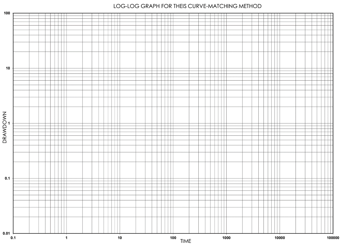
Figure 43 ‑ Blank log‑log graph paper with same scale and extent as type curve shown in Figure 44 for curve‑matching.
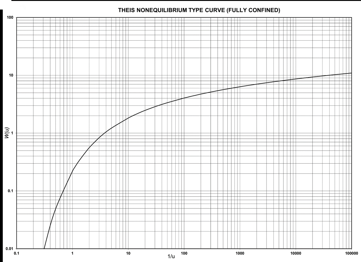
Figure 44 ‑ Theis non‑equilibrium type curve for non‑leaky (i.e., fully) confined aquifers.
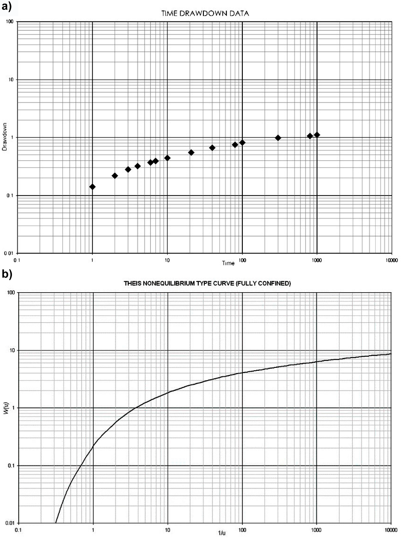
Figure 45 ‑ Example data for curve‑matching method: a) time‑drawdown data from an aquifer test; b) Theis non‑equilibrium type curve for non‑leaky (i.e., fully) confined aquifers.
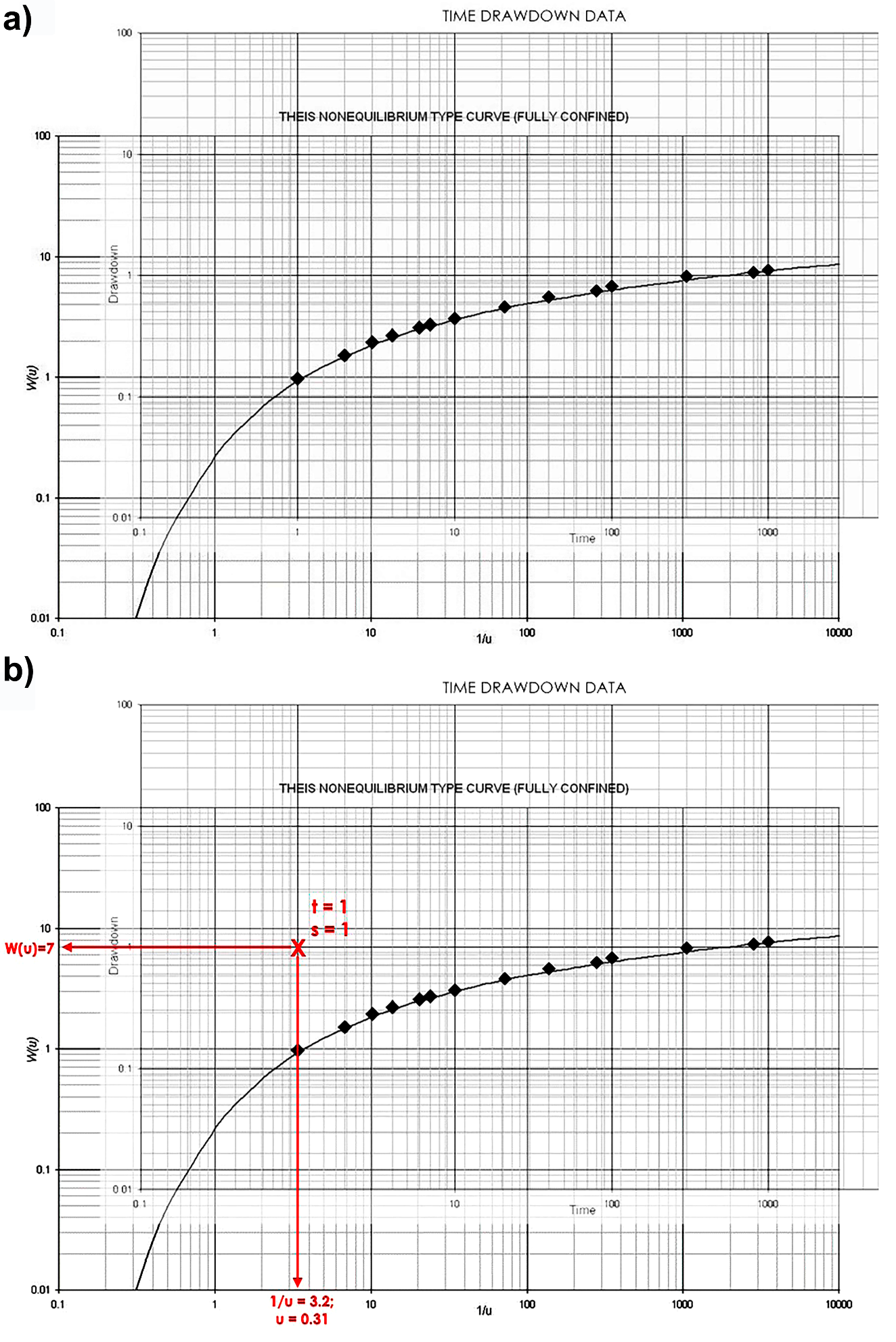
Figure 46 ‑ Example of curve‑matching method: a) plotted data overlain on type curve with best match of the data to the type curve; b) match point t (time) = 1 and s (drawdown) = 1 on data graph corresponds to W(u) = 7 and u = 0.31.
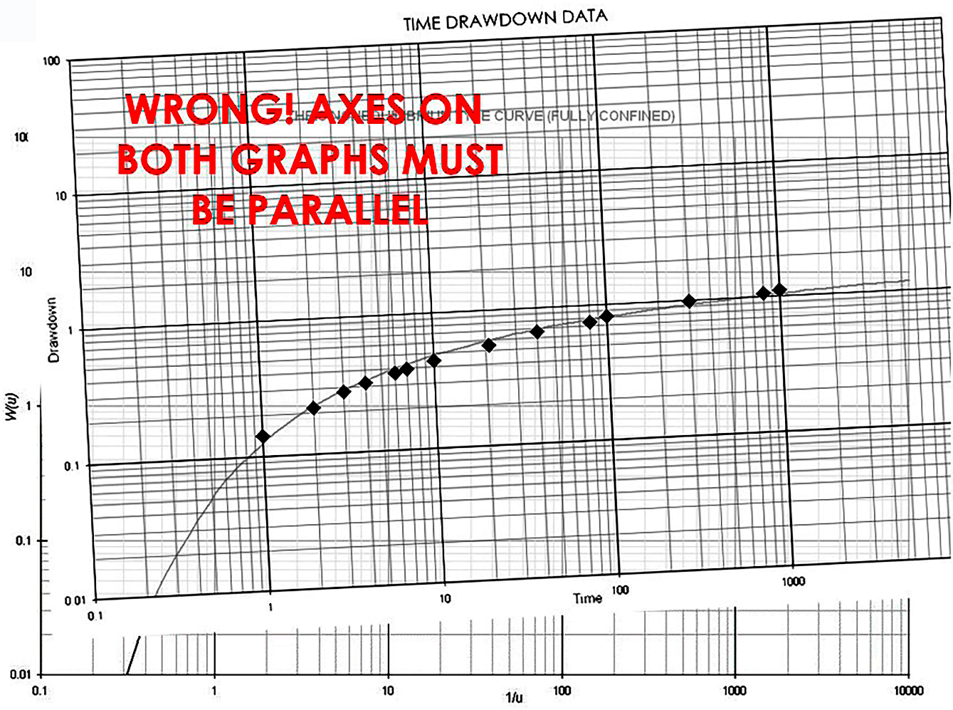
Figure 47 ‑ Example of incorrect curve‑matching due to failure to properly align the axes.
Leaky Confined and Unconfined Methods
As shown in Figure 40, the drawdown curve for a leaky confined aquifer will not follow the same shape as a non‑leaky confined aquifer; therefore, drawdowns from a leaky confined aquifer will not match the Theis non‑leaky type curve due to reduced drawdowns caused by the addition of water to the aquifer through the leaky confining layer. Hantush and Jacob (1955) and Walton (1960) developed curve‑matching methods that are like the Theis method but include additional type curves and an additional term in the well function that accounts for the contribution of interformational leakage. A version of the Walton type curves is provided as Figure 48.
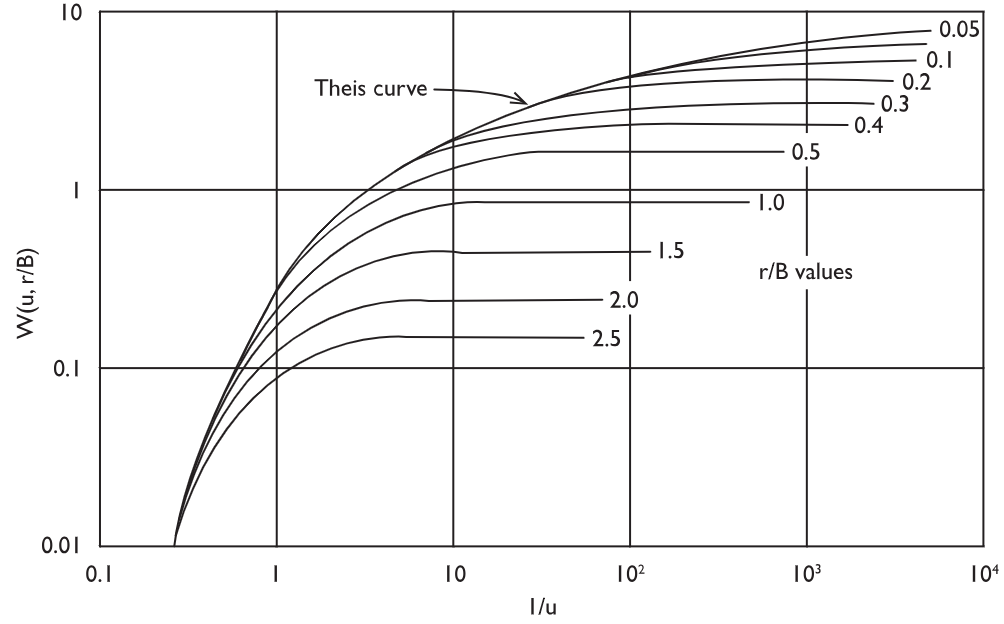
Figure 48 ‑ Theoretical type curves of W(u,r/B) versus 1/u for a leaky aquifer (from Freeze & Cherry, 1979; modified from Walton, 1960).
In an unconfined aquifer, the drawdown response has three separate parts to it which result in a distinctive shape shown in Figure 42. Neuman (1975) developed a similar curve‑matching method in which the well function is composed of three separate arguments, one for each of the drawdown stages. A version of the Neuman type curves is presented as Figure 49.
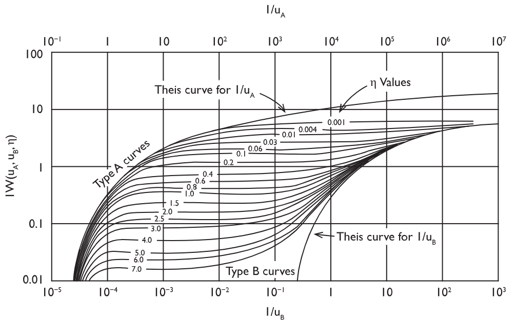
Figure 49 ‑ Theoretical type curves of W(uA, uB, η) versus 1/uA and 1/uB for an unconfined aquifer (from Freeze & Cherry, 1979; modified from Neuman 1975).
The leaky and unconfined methods are discussed in more detail in sections 9 and 10 of An Introduction to Hydraulic Testing in Hydrogeology: Basic Pumping, Slug, and Packer Methods↗ by Woessner and others (2020), as well as in Analysis and Evaluation of Pumping Test Data (2nd edition)↗ by Kruseman and others (2000). Both books are available as free downloads from The Groundwater Project. Readers are encouraged to review these books for more information.