
3.3 Permeability
Porosity is an important parameter in hydrogeology; however, it is not the only quantity that we need to understand to characterize groundwater systems. Different materials transmit fluids with varying degrees of difficulty. The ease with which a porous medium transmits fluid is called the permeability.
Darcy’s Law
Henry Darcy (1856) experimented with fluid flow through a pipe filled with sand (Figure 14a) as part of a larger project to design filtration systems for the public fountains of Dijon, France. He forced water through the pipe under a hydraulic head—that is, he filled up a reservoir at a higher elevation than the pipe and allowed gravity to drive water through the sand—then he measured:
- the rate of discharge through the pipe ([latex]Q[/latex]); and
- the loss in head ([latex]dh[/latex]) across some length of the pipe ([latex]dl[/latex]).
He concluded that discharge of water through the pipe is directly proportional to the energy loss and inversely proportional to the length of the path of flow (Figure 14b). Or, if we call the loss in head over a length the hydraulic gradient, he found that the discharge is directly proportional to the hydraulic gradient. This statement is expressed mathematically as Equation (22).
| [latex]\frac{Q}{A} \propto \frac{dh}{dl}[/latex] | (22) |
|---|
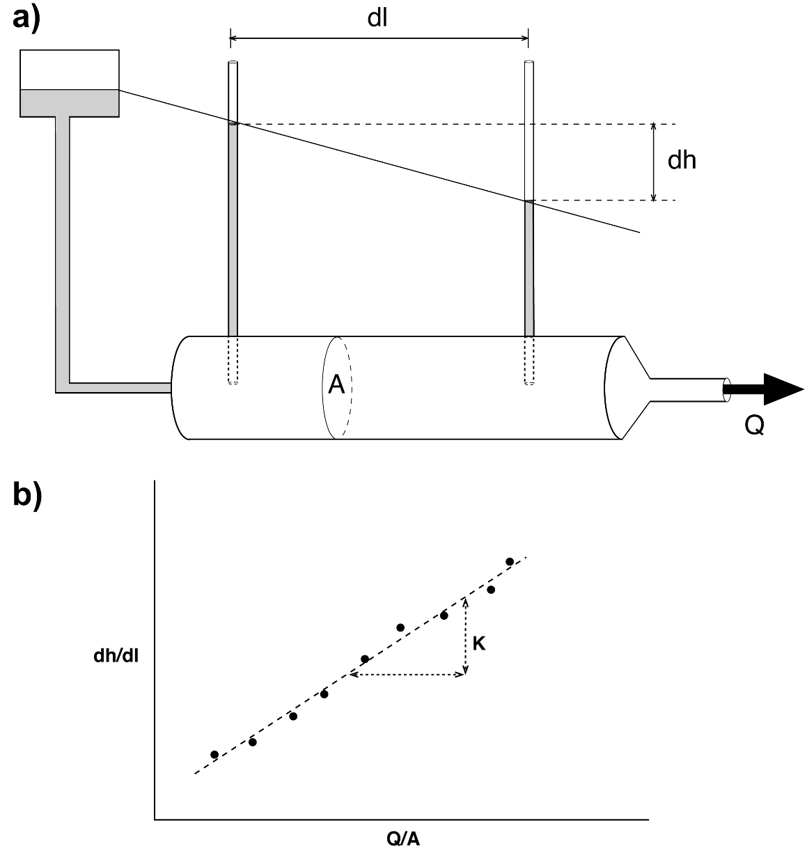
Figure 14 ‑ a) Darcy tube; b) graph showing experimental results.
What Does This Mean?
Notice that the data fall on a relatively straight line when graphed, meaning that the proportionality is linear. Whenever you have a relationship where one quantity is linearly proportional to another, the slope of the line allows you to set the two quantities equal to each other. In mathematical terms, this slope is a constant of proportionality or a coefficient of proportionality. In this specific equation, we call the constant the hydraulic conductivity ([latex]K[/latex]). Inserting [latex]K[/latex] and rearranging the equation to solve for Q gives us Darcy’s law, as expressed by Equation (23).
| [latex]Q = - KA\frac{dh}{dl}[/latex] | (23) |
|---|
where (parameter dimensions are dark green font with mass as M, length as L, time as T):
| [latex]Q[/latex] | = | volumetric discharge (L3T-1) |
|---|---|---|
| [latex]K[/latex] | = | hydraulic conductivity (LT-1) |
| [latex]A[/latex] | = | area perpendicular to flow (L2) |
| [latex]dh[/latex] | = | difference in head (L) |
| [latex]dl[/latex] | = | distance over which dh occurs (L) |
If we divide through by the cross‑sectional area, the volumetric discharge reduces to a 1‑dimensional discharge (i.e., velocity) called the Darcian velocity ([latex]q[/latex]), as shown by Equation (24).
| [latex]q = - K\frac{dh}{dl}[/latex] | (24) |
|---|
Darcian velocity is also called the specific discharge. This value should not be considered to represent the actual velocity of groundwater flow as not all of the cross-sectional area perpendicular to flow is actually open and available for fluid flow. This is discussed in more detail in Section 3.3.7.
When we deal with aquifers, we often use a quantity called the transmissivity ([latex]T[/latex]), which is defined as the hydraulic conductivity multiplied by the saturated thickness of the aquifer ([latex]b[/latex]), as expressed by Equation (25).
| [latex]T = Kb[/latex] | (25) |
|---|
The importance of this value will become evident in later sections of this book; for now, it is useful to be aware of the definition of the term.
In summary, hydraulic conductivity is a quantity that characterizes the ease with which water moves through a porous medium. Darcy’s study indicated that different porous media (i.e., different types of sand with different grain size distributions) have different [latex]K[/latex] values, indicating that each media has a distinct value of [latex]K[/latex]. It is important to realize, however, that this relationship is for water specifically; if we are studying some other fluid—petroleum, high‑salinity brine, molasses, and so on—we need to use a different coefficient.
Permeability for Other Fluids
The ease with which a fluid moves through a porous medium is dependent on:
- properties of the media (size of pores and connectivity); and
- properties of the fluid (density and viscosity).
The hydraulic conductivity, as measured and characterized by Darcy’s law, is for water. This quantity not only characterizes the properties of the media, but it also contains the properties of the fluid moving through that media. Because of this, a hydraulic conductivity obtained for a sand by using water as the fluid in Darcy‘s apparatus cannot be used to calculate the flow rate of a different fluid—for example, motor oil or mercury. This is not a big deal in most hydrogeology problems, since we generally deal with water in near‑surface environments, but it does concern us if we are dealing with multiple phases, or types of fluids—for example, oil and water—in an aquifer. To handle such multi‑phase flow problems we use a quantity called the intrinsic permeability ([latex]k).[/latex] This value is a quantity that characterizes the ease with which any fluid flows through a porous medium, and only characterizes the porous medium itself. Equation (26) shows how intrinsic permeability can be used in Darcy’s law.
| [latex]Q = k\frac{\rho_{fluid}\ g}{\mu_{fluid}}[/latex] | (26) |
|---|
where (parameter dimensions are dark green font with mass as M, length as L, time as T):
| [latex]k[/latex] | = | intrinsic permeability (L2) |
|---|---|---|
| [latex]\rho_{fluid}[/latex] | = | density of the fluid (ML-3) |
| [latex]g[/latex] | = | gravitational acceleration (LT-2) |
| [latex]\mu_{fluid}[/latex] | = | viscosity of the fluid (ML-1T-1) |
This equation requires that the user specify the properties of the fluid—that is, density and viscosity. Otherwise, it is the same as Darcy’s law. The hydraulic conductivity and the intrinsic permeability are related as shown by Equation (27).
| [latex]k = K\frac{\mu_{fluid}}{\rho_{fluid}\ g}[/latex] | (27) |
|---|
Other Famous Equations Analogous to Darcy’s Law
The basic ideas conveyed by Darcy’s law are:
a) discharge is driven by a gradient;
b) discharge is linearly proportional to a gradient; and
c) there is a constant of proportionality that characterizes the ease with which water flows through the system (a conductivity parameter).
Throughout the natural sciences we find numerous other physical processes that are mathematically identical to groundwater flow in that they have the same three properties. Examples including:
- heat flow (Fourier’s Law);
- electrical flow (Ohm’s Law); and
- diffusive flow of solutes (Fick’s Law).
Each one of these equations has a discharge rate, a gradient or potential, and a constant of proportionality that represents conductivity. The importance of this is that we can use solutions from these other sciences and apply them to groundwater flow problems. This is discussed using a specific example in the section on Well Hydraulics (Section 7).
The Limits of Darcy’s Law
Although Darcy’s law is regarded as a fundamental relationship in the Earth sciences, it has limitations, and there is a range of conditions over which it is valid.
Upper limit
One of the assumptions inherent in Darcy’s law is that the flow is laminar. Darcy’s law is not valid above the onset of turbulence in the system because the discharge is no longer linearly proportional to the gradient.
Lower limit
The lower limit of Darcy’s law occurs at the threshold gradient, where fluid viscosity is too strong for the gradient to overcome the resistance to flow.
Applicability
Darcy’s law is still widely used because
- groundwater systems rarely become turbulent, and
- at gradients near the threshold gradient, flow is generally so small that it can be ignored.
Thought Question 4: In what geologic situations might we be concerned about groundwater flow exceeding the limits of Darcy’s law?
Measuring Permeability
Understanding permeability is one thing; measuring it is another matter. Unfortunately, no one has developed a simple permeability meter with a digital display that you can point at a rock or sediment and instantly measure the permeability. Instead, we have a variety of ways of measuring permeability, both in the field and in the laboratory. These methods generally involve forcing fluid through a sample of the material, measuring the head loss and discharge rate, and calculating permeability from the measurements.
Permeameters or Darcy tubes are like the apparatus shown in in Figure 14a. The procedure involves filling the tube with a sample, running water through the sample under a constant head in the reservoir, reading the values of head loss (dh) and discharge (Q), then using those measurements and Darcy’s law to calculate hydraulic conductivity. Permeameters are generally used for unconsolidated (i.e., loose) material like sand or gravel that can be packed into a column or minimally disturbed cores of the material. Some permeameters are designed to measure permeability in small cores taken from consolidated (i.e., solid) rock.
Gas permeameters are like regular permeameters except they use a gas (usually nitrogen) as the fluid instead of water. These can be portable for field use or set up in a laboratory. Gas permeameters require additional mathematical adjustments to account for the compressibility of air.
Well/piezometer tests, also known as pumping tests or hydraulic tests, are tests performed in the field on wells or piezometers. These tests generally involve pumping water at a known rate while simultaneously monitoring water levels in the pumping well and, if possible, any nearby wells. Wells can also be tested by displacing a known volume of water from the well and monitoring the recovery of the water levels over time; this is known as a slug test. More information on pumping and slug testing can be found in An Introduction to Hydraulic Testing in Hydrogeology: Basic Pumping, Slug, and Packer Methods↗ by Woessner and others (2023), which is available as a free download from The Groundwater Project. Well testing is discussed in more detail in Section 8.
Numerous researchers have developed empirical equations to calculate permeability—that is, equations expressing relationships based on experimental data, as opposed to equations derived from first principles. The empirical equations are based on observed correlations between permeability and properties of the rock, primarily grain size distributions, average grain size, or effective grain size. In general, larger grain size is correlated with higher permeability; however, the relationship is not that simple. As indicated by Figure 13c and Figure 13d, the distribution of grain sizes can be just as significant as overall size, with well‑sorted sediments—that is, very little variation in grain size—correlated with greater permeability.
Permeability can also be estimated using inverse methods, which involve using data collected in the field—for example, water levels in wells, groundwater flow rates from discharge to springs and streams, and dimensions of the aquifer—to estimate, or “back out”, permeability values using numerical models and automated model calibration techniques.
Fluid Velocity
We have stated that dividing the Darcy equation by the cross‑sectional area reduces the volumetric discharge ([latex]Q[/latex]) down to a one‑dimensional discharge ([latex]q[/latex]) that we call the specific discharge or Darcian velocity. In reality, however, groundwater is not flowing through the entire cross‑sectional area; it is only flowing through the pore spaces, which make up a percentage of the total area. We must therefore modify the specific discharge by dividing it by the effective porosity to get a value called the average linear velocity ([latex]v[/latex]), which is a more accurate characterization of the groundwater velocity. Calculation of specific discharge is shown by Equation (28).
| [latex]v = \frac{q}{\varphi_{eff}}[/latex] | (28) |
|---|
It is common for practicing hydrogeologists to use estimates of hydraulic conductivity, effective porosity, and hydraulic gradient to calculate an average linear velocity and then use that velocity to develop estimates about travel times of contaminants in the aquifers that they study. These calculated travel times are then used to develop plans for remediation (i.e., cleaning up) of groundwater contamination at sites that have been impacted by leaking tanks or accidental releases of contaminants. Several decades of experience in assessing and remediating groundwater contamination has shown that travel time estimates based on the average linear velocity are almost always much longer than observed travel times, which means that contaminants generally move much faster than the average linear velocity estimates. Exercise 5⮧ provides an opportunity to make calculations related to groundwater velocity.
These observed discrepancies are likely associated with the fact that the true velocity of the groundwater varies from point to point in an aquifer depending on the size of the pores, the tortuosity of the flow paths, and constriction at the pore throats. If one were able to measure flow velocities at many points in an ideal aquifer, one would see very fast velocities at a few locations, very slow to even stagnant water in other locations, with a wide range of velocities in between. Plotting a frequency histogram of these velocities would likely show us a normal distribution centered around the average linear velocity calculated by Equation (28). However, given the observation that contaminants arrive sooner than expected, we can conclude it is common for contaminants to move along paths with higher velocities. Thus, we need to be cautious about using the average linear velocity to estimate travel times. A discussion of alternative methods for developing meaningful estimates of groundwater velocity is beyond the scope of this book. Readers are encouraged to review Groundwater Velocity↗ by Devlin (2020), available from The Groundwater Project as a free download or can be read online.
Thought Question 5: How is it that the variations in actual groundwater velocity can result in faster than expected arrival of contaminants at a potential receptor (i.e., a downgradient water well) versus estimates derived from calculating the average linear velocity?
Permeability Distributions in Aquifers
As mentioned, the definitions of scalar, vector, and tensor quantities in mathematics are:
- scalar quantities have magnitude only;
- vector quantities have magnitude and direction; and
- tensor quantities have magnitude that varies with respect to direction.
Permeability is a tensor quantity. Not only does it vary from place to place, but it also varies with respect to direction. We can use two vectors to graphically represent a permeability tensor and to describe the variations in permeability throughout a system.
When we talk about variations of permeability in an aquifer, we use the terms heterogeneity and anisotropy. Heterogeneity is variation in a parameter with respect to location within a system. Anisotropy is variation in a parameter varies with respect to direction.
Figure 15 graphically shows the relationship between these two terms. It is important not to use these terms interchangeably—each has a specific meaning.
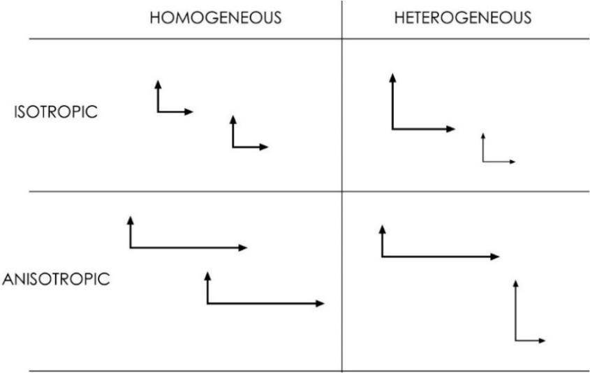
Figure 15 ‑ Graphical representation of the relationship between heterogeneity and anisotropy.
It should be noted that all aquifers and groundwater systems have some degree of heterogeneity with respect to permeability. It is essentially impossible to determine the actual distribution of permeabilities in an aquifer, so it is common for practicing hydrogeologists to assume that the system can be approximated as a homogeneous system with a single permeability or a heterogeneous system with a small number of homogenous permeability zones. Anisotropy in aquifer systems is generally associated with the natural layering of geologic formations such that permeability in the vertical direction is generally less than that in the horizontal direction. Anisotropy is also associated with systematic fractures (e.g., fault zones, joint sets) and is also associated with certain depositional environments (e.g., fluvial). More information on the impact of fractures on groundwater flow can be found in Fractures and Faults in Sandstone and Sandstone‑Shale/Mudstone Sequences and Their Impact on Groundwater↗ by Aydin and others (2023), section 5.6 of Hydrogeologic Properties of Earth Materials and Principles of Groundwater Flow↗ by Woessner and Poeter (2020), and Structural Geology Applied to Fractured Aquifer Characterization↗ by Fernandes and others (2023). Each book is available as a free download from The Groundwater Project.
Statistical Distribution
Permeability is a quantity that varies over 19 orders of magnitude! When we are studying an aquifer and we measure many permeabilities in that aquifer, our measurements typically cover several orders of magnitude. When multiple measured aquifer permeability values are available it is common to take an average of those values and use that average to perform calculations or develop models. Since permeability generally ranges across several orders of magnitude, we must be careful when averaging permeabilities to get a single value to characterize an aquifer.
In mathematics there are several ways of calculating a mean (i.e., average) for a set of data. The relevant methods for us are listed here.
- Arithmetic mean: Add up the values and divide by the number of measurements.
| [latex]\frac{\sum_{i = 1}^{n}\left( k_{i} \right)}{n}[/latex] | (29) |
|---|
- Geometric mean: Add up the logs of each value and divide by number of measurements and raise ten to that power.
| [latex]10^{\left( \frac{\sum_{i = 1}^{n}\left( \log\left( k_{i} \right) \right)}{n} \right)}[/latex] | (30) |
|---|
- Harmonic mean: Divide the number of measurements by the sum of the reciprocal of each measurement.
| [latex]\frac{n}{\sum_{i = 1}^{n}\left( \frac{1}{k_{i}} \right)}[/latex] | (31) |
|---|
We are generally used to dealing with quantities that follow normal distributions, in which the values are distributed around an arithmetic mean value. Examples of normally distributed quantities include the heights of people in a population, the grades of students in a large class, and variations in air temperatures over time at a single location. Permeability is a log‑normally distributed value (Figure 16). A log‑normal distribution means that the logarithm of permeability is distributed around a mean, and if we calculate an arithmetic mean for log-normally distributed data we are likely over‑estimating the value that could serve as a representative value for the entire formation. The implication is that we should not use the arithmetic mean of multiple measured permeability values to characterize the permeability of an aquifer; instead, it is more appropriate to use a geometric mean—that is, average the logarithms rather than the actual values.
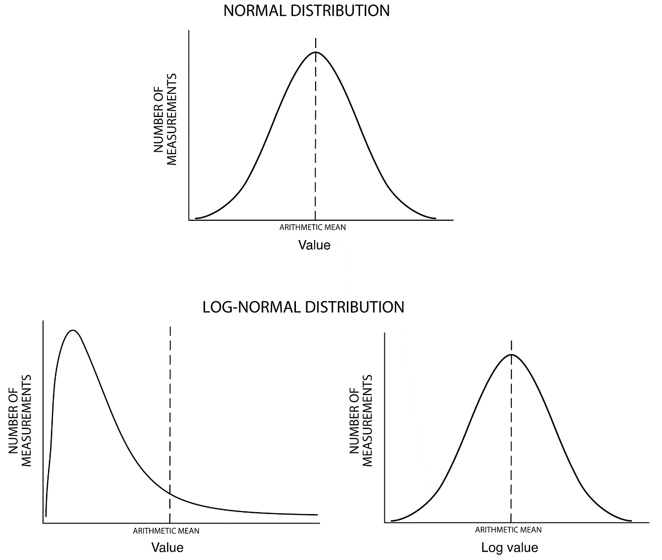
Figure 16 ‑ Normal versus log‑normal distribution.
A more detailed discussion of the properties of porous media and the relationships between those properties and groundwater flow can be found in Hydrogeologic Properties of Earth Materials and Principles of Groundwater Flow↗ by Woessner and Poeter (2020) which is available from The Groundwater Project as a free download or can be read online.