
10.3 Specific Types of Groundwater Flow Models
We have defined the word model and presented reasons for using models. Now, we discuss the various types of models used to simulate groundwater flow in more detail.
Qualitative Models
Simple groundwater contour maps and flow nets are geometric models that provide qualitative information about groundwater flow processes. For example, a groundwater contour map can be used to infer the direction of groundwater flow and identify changes in hydraulic gradient throughout the mapped area, which can in turn be used to identify heterogeneities in aquifers.
Conceptual Hydrogeological Models
All the aspects of a groundwater flow system described in Sections 1 through 9 can be used to develop a summary of the relevant aspects of an aquifer or groundwater flow system. This summary is called a conceptual hydrogeological model (CSM). A CSM contains information about aquifer structure; aquifer boundaries; recharge and discharge mechanisms along with estimates of recharge and discharge rates; hydrostratigraphic units that make up the various components of the aquifer and associated confining units along with their properties; interpretations of groundwater flow paths; and projections about future changes to the aquifer (e.g., pumping from wells, effects of climate change). A CSM is the first objective of major aquifer studies, and developing a reliable CSM is a prerequisite for developing the process models described in the subsequent sections of this book.
Physical or Analog Models
Physical models that simulate groundwater flow include tanks full of sand or other sediments with input pipes and drains that can be used to simulate flow through porous media. Physical models made from layers of sand or clay have also been used extensively in structural geology problems. Another physical model simulating fluid flow used two glass plates sandwiched together with small channels etched on the surface of the plates.
Analog models use the similarity between Darcy’s law and other physical processes to model fluid flow. The most popular way of doing this is with electrical circuit models in which the flow of current represents the flow of groundwater, the changes in voltage represent the changes in head, and the resistance of the conductors represents the hydraulic conductivity, as in Equation (89)and Equation (90). Capacitors can be added to the circuit to simulate aquifer storage.
| Darcy’s law: [latex]q = - K\frac{dh}{dl}[/latex] | (89) | |
|---|---|---|
| Ohm’s law: [latex]I = - \frac{1}{R}\frac{dV}{dl}[/latex] | (90) |
where (parameter dimensions are dark green font with mass as M, length as L, time as T):
| [latex]q[/latex] | = | water flow through a conductive porous medium |
|---|---|---|
| [latex]I[/latex] | = | current flow through an electrical conductor |
| [latex]K\ and\ 1/R[/latex] | = | proportionality coefficients (K is hydraulic conductivity and R is electrical resistance, which is the inverse of electrical conductance) |
| [latex]dh/dl[/latex] | = | head drop across the conductive porous medium |
| [latex]dV/dl[/latex] | = | voltage drop across the electrical conductor |
Mathematical Models
Any equation that represents a physical process is a model of that process. Darcy’s law is a model that represents the flow of groundwater in one dimension. Because it is a model, it tells us something about how the system behaves—that is, flow is linearly proportional to the hydraulic gradient—and it can be used to make predictions about the system—for example, to calculate travel times and flow velocities.
A good deal of this book talks about the basic equations that govern the flow of groundwater in a three‑dimensional, transient system. Specific solutions to this equation can be developed and used simulate groundwater flow in flow systems and aquifers. The basic groundwater flow equation is shown as Equation (91).
| [latex]\frac{\partial\left( K_{x}\frac{\partial h}{\partial x} \right)}{\partial x} + \frac{\partial\left( K_{y}\frac{\partial h}{\partial y} \right)}{\partial y} + \frac{\partial\left( K_{z}\frac{\partial h}{\partial z} \right)}{\partial z} = S_{s}\frac{\partial h}{\partial t}[/latex] | (91) |
|---|
This equation describes the flow of groundwater and change in storage with time at a single point in a flow system. If we apply boundary conditions to this partial differential equation, then for simple geometry and homogenous properties we can solve the equation for a specific flow system using an analytical solution.
The problem with using this equation for practical groundwater flow problems is that parameters and boundary conditions vary in space and time, and we have an infinite number of points in any system—and therefore an infinite number of equations to solve—and the heads and fluxes at each point are dependent upon the heads and fluxes at all the surrounding points. We can’t simultaneously solve an infinite number of equations, so we must simplify the system in some way and then use that simplification to solve the problem and model the system. There are many methods for solving equations like these, but they are variations of two basic approaches to solving partial differential equations: analytical and numerical.
Analytical Solutions
One can consider a specific scenario, develop some assumptions that simplify the system, and then use those assumptions to develop an analytical solution to the equation. The Theis equation is an example. Theis considered a specific situation—radial flow to a well—with several simplifying assumptions—homogeneity, constant thickness, infinite extent, a fully penetrating well of infinitesimal radius, and so on—and derived an equation that directly solves for the drawdown in the aquifer at some distance from a pumping well and at some time after pumping started.
Analytical solutions are advantageous because they are easy to use—since they can be solved directly—and they give unambiguous results at any of the infinite number of locations within the system. However, they are limited because they require simplification of the systems, and so they are not always applicable to solving meaningful problems. Also, we may have a specific situation for which we want to derive a solution, but the situation may be so complex that a direct solution isn’t possible. In such cases we turn to numerical approaches.
Numerical Solutions
If an analytical solution is not possible, an alternate approach to solving the equation is to develop an approximation called a numerical solution. The basic procedure for developing a numerical solution is to first determine the problem domain—the geometry and volume of the system— and its boundary conditions, then reduce the infinite number of points—and corresponding equations—in the system to a finite number of points, and then use an iterative method to solve the equations at those points.
The process of reducing the system to a finite number of points is called discretization—that is, making a continuous function into a discrete function. An example is shown in Figure 73. In this example, an alluvial aquifer that contains an infinite number of points is discretized by superimposing a regular grid of six columns and eight rows containing 48 points, or nodes. Each point contains a version of the groundwater flow equation that calculates hydraulic head at each point based on the values of head at the surrounding points. The grid also has boundary conditions based on the physical boundaries of the model—the river and the granite fault block—and the northern and southern extent of the study area that are symmetry boundaries (Figure 61).
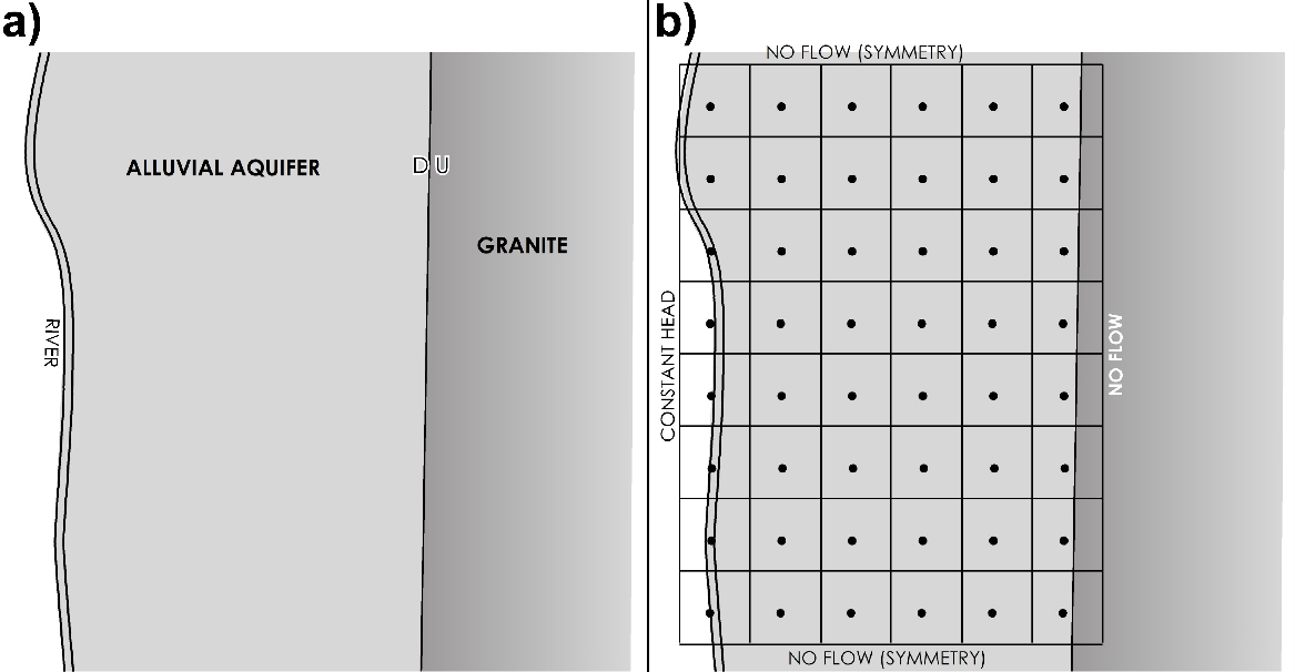
Figure 73 – a) Map of an alluvial aquifer, bounded by a river to the west and a fault‑block granite to the east; and b) discretization of the alluvial aquifer with boundary conditions and model nodes.
Once the model grid has been discretized and the equations are added to each node, an initial value of head is assigned to each node and the set of equations are solved. However, the value of head at each node is dependent upon the value at each of the four surrounding nodes (Figure 74). If the head at a given node is calculated based on the heads at the surrounding nodes, then when the head is calculated at the next adjacent node, its head changes so the head at the first node needs to be recalculated.
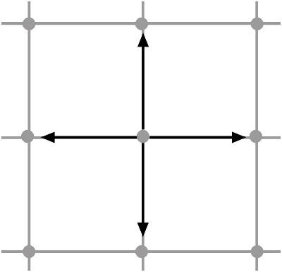
Figure 74 ‑ The value at any node is dependent upon the values at the surrounding nodes.
This is where the numerical part of the method is applied. This is done by assigning initial heads to all nodes, then using matrix solutions—which can be thought of in a simplified sense as starting at one corner of the model, calculating a head at that node, then systematically moving across the row to calculate the value at each node. The same process is then applied to the next row, then the next, and so on, until all nodes have been calculated and the value at each node has been recorded. The process is then repeated, and the values from the second set of calculations—that is, the second iteration—are compared to the first set of calculations and the difference between each set is calculated. This process is then repeated multiple times until the change in head from one iteration to the next is so small that it can be considered negligible. At this point, the model has converged on an approximate solution. Simple models with well‑chosen initial heads can converge in only a few iterations, while complex models can take hundreds or even thousands of iterations to converge. Complex models can also experience mathematical instability, which in turn results in models that never converge.
This iterative process is where the importance of modern computers comes in. A person using a pencil, paper, and a hand‑held calculator could take years to calculate and solve a simple model with only a few nodes. Developing numerical models was not feasible until the development of digital computers that can do lots of calculations in incredibly short time. Computing power is so great now that inexpensive desktop computers can solve sophisticated models in a relatively short time. However, the processing time can become significant if there is a lot of detail in the model, or if an automated calibration or uncertainty analysis is applied to a large model.
Discretizing a system involves decisions concerning how much detail needs to be built into the model, and these decisions are based in many ways on the model objectives and the amount of detail required for the results. The more nodes that are included in the model grid, the more computationally intensive the model. Also, more complexity increases the possibility of numerical instability and a model that won’t converge. In many cases, simpler models are better because there is less estimation and uncertainty, and frequently they are sufficient to provide the information that we need.