
8.9 Multiple Wells, Boundaries, and Image Wells
In Section 6 we introduced the concept of boundary conditions relative to how boundaries affect flow lines and equipotential lines on flow nets. In this section we discuss how boundary conditions affect drawdowns induced by pumping wells and relate that to the influence of multiple pumping wells on a single point in an aquifer.
Superposition
As we previously demonstrated, pumping from a well at a constant rate for a certain amount of time will result in a certain amount of drawdown at an observation well located some distance away from the pumping well. Now let’s consider what would happen to the water levels at the observation well if there are multiple pumping wells in the general vicinity of the observation well (Figure 54).
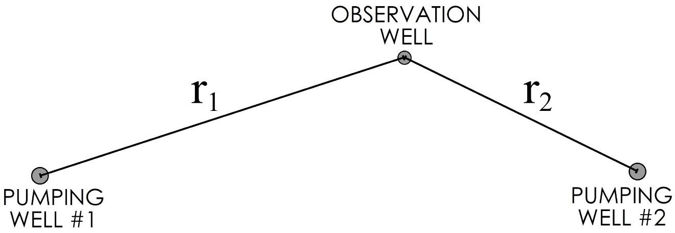
Figure 54 ‑ Map view of observation well influenced by multiple pumping wells.
In this case, each pumping well induces a cone of depression in the aquifer, and the cones of depression overlap at the observation well and throughout the aquifer. Since each pumping well is affecting the observation well, the resulting drawdown at the observation well will be greater than it would for a single pumping well. The effect of pumping from one well on the cone of depression developed by a second pumping well is called well interference. In this case, the total drawdown experienced by the observation well is the sum of the drawdowns induced by each pumping well. This is the principal of superposition. It is applicable for near-linear conditions such as those in a confined aquifer, or in unconfined aquifers when the drawdown is relatively small compared to the saturated thickness of the aquifer.
It is therefore relatively easy to calculate the drawdown in an observation well influenced by multiple pumping wells, provided that the aquifer [latex]T[/latex] and [latex]S[/latex] are known with confidence and if one is calculating drawdowns at a specific point in time. The procedure involves calculating the drawdown from pumping well #1 at distance [latex]r_{1}[/latex], then calculating the drawdown from pumping well #2 at [latex]r_{2}[/latex], then summing the two values to get a total drawdown. The procedure is illustrated by Exercise 16⮧.
Use of Image Wells to Represent Boundaries
This concept of superposition is useful for calculating the drawdowns induced by multiple pumping wells. It can also be used to evaluate drawdowns affected by hydraulic boundaries in the aquifer. Let us consider two basic types of hydraulic boundaries—constant head boundaries and no‑flow boundaries—and the specific influence that each of these have on the drawdown response in an observation well (Figure 40 and Figure 41). As previously discussed, constant head boundaries essentially add water to the system when head inside the boundary declines so less water is removed from storage and thus drawdowns are not as large (Figure 40). In the case of no‑flow boundaries, less area is available around the well to contribute water from storage so the same volume of pumped water comes from a smaller area of the aquifer thus drawdowns are larger. These boundary impacts are equivalent to the effect a second pumping well would have on an observation well in an unbounded aquifer. This equivalence can be used to calculate the effect of a boundary on drawdowns from a pumping well through the application of image wells.
If the location of a linear boundary and the transmissivity and storativity of the aquifer are known with some confidence, the drawdown at an observation well can be calculated by mathematically placing an imaginary pumping well, the image well, in the aquifer an equal distance from the boundary, but on the opposite side of the boundary. To represent a hydraulic boundary the image well is an injection well (Q is negative), while a no-flow boundary is represented with a pumping well (Q is positive). The drawdown at the observation well is then calculated as the sum of the calculated drawdowns due to the pumping well and the image well.
An example of a pumping well near a no‑flow boundary is shown in map view (Figure 55) and in cross‑sectional view (Figure 56a). The pumping well is located some distance rboundary away from the edge of the aquifer. The boundary created by the uplifted block of granite reduces the area around the well where water can be removed from storage to flow to the pumping well. This can be represented as a second pumping well in an unbounded aquifer an equal distance from the boundary and pumping at the same rate (Figure 56b). This image well creates the exact same drawdown as the pumping well along the line between them. With the same water level on both side of the boundary, the gradient is zero which is the definition of a no-flow boundary. The drawdown at the observation well located near the boundary is the sum of the calculated drawdown from the pumping well, at distance [latex]r_{real}[/latex] and the calculated drawdown from the imaginary well, or image well, at distance [latex]r_{image}[/latex].
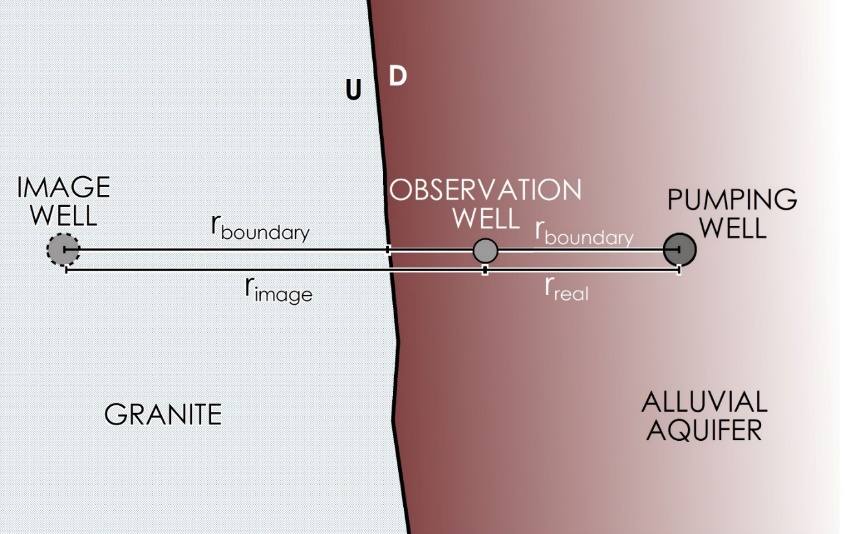
Figure 55 ‑ Map view of pumping well at a no‑flow boundary with an associated image well.
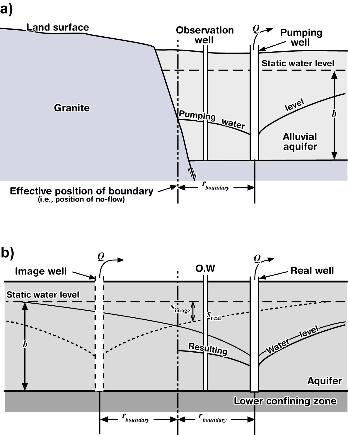
Figure 56 ‑ a) Cross‑section of the system shown in Figure 55; b) equivalent system with unbounded aquifer and an image well.
The same procedure can be done to evaluate drawdowns near a constant head boundary (Figure 57 and Figure 58a); the only difference is that a constant head boundary is supplying additional water to the system which results in less drawdown because less water is removed from storage to satisfy the pumping well. In that case, the image well is an injection well with a negative Q (Figure 58b) that produces a negative s so it produces “drawup” such that the calculated drawdown associated with the image well is subtracted from the pumping well drawdown (Exercise 17⮧).
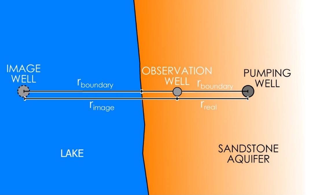
Figure 57 ‑ Map view of pumping well at a constant head boundary with an associated image well.
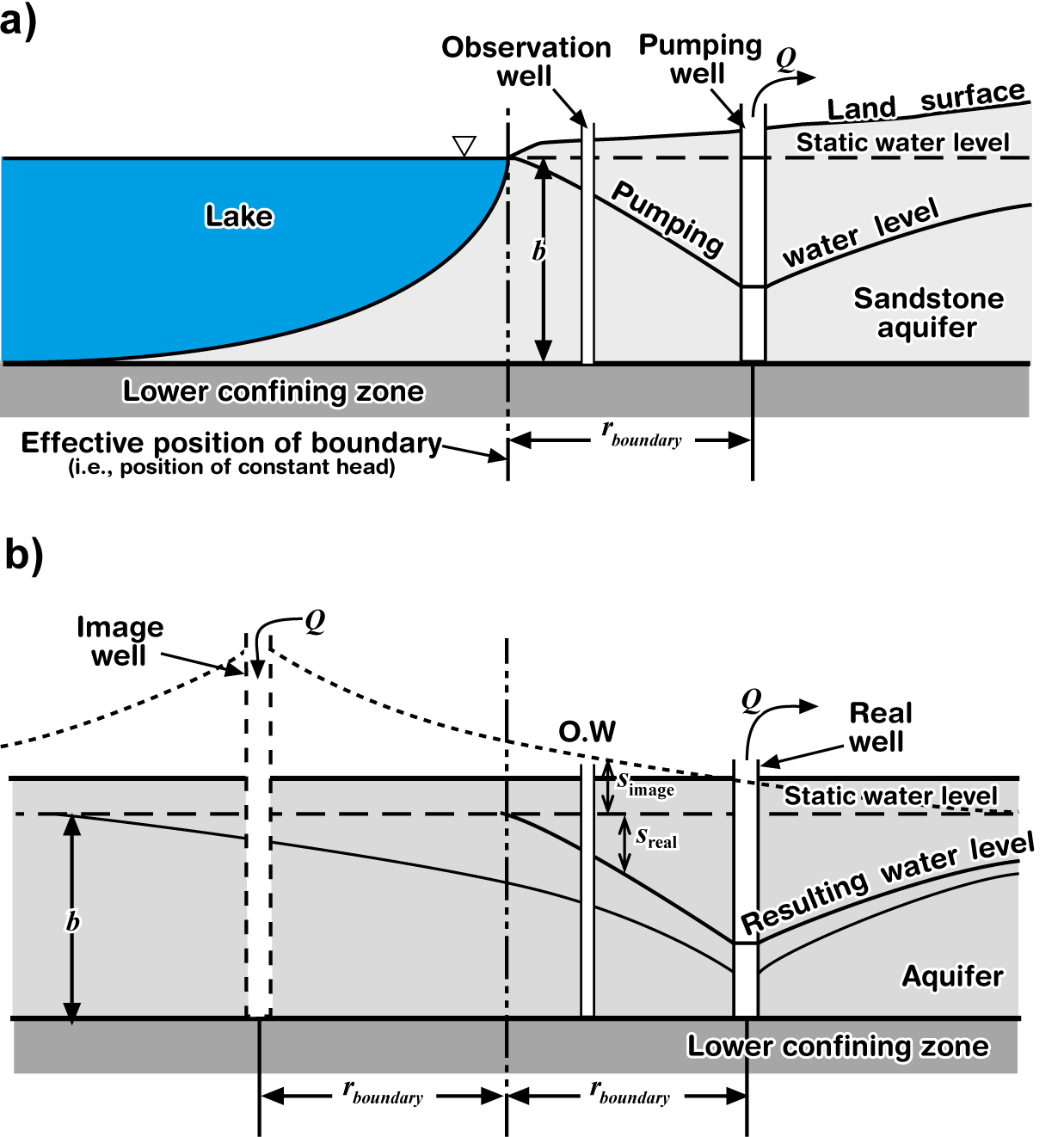
Figure 58 ‑ a) Cross‑section of a system shown in Figure 57; b) equivalent system with unbounded aquifer and an image well.