
8.7 Well Loss and Well Efficiency
Well efficiency refers to the difference between the expected performance of a well (i.e., the expected drawdown in response to pumping at a specific rate for a given amount of time) and the actual performance. In other words, it refers to the difference between the drawdown we expect to see in the aquifer at the pumping well and the actual drawdown measured in the well during pumping. To understand well efficiency, we have to revisit the idea that hydraulic head is a measure of fluid energy, and that drawdown is actually measuring a reduction in fluid energy—that is, a decline in head—resulting from stressing an aquifer—that is, pumping water from the aquifer.
Drawdown and Fluid Energy
Pumping from a well draws water into the well from the aquifer, which in turn causes water to flow from farther away in the aquifer towards the well. This reduces pressure in the aquifer, which in turn reduces the pressure head component of energy in the formation causing a drop in hydraulic head—that is, drawdown—and formation of a cone of depression in the aquifer around the well. The amount of energy loss for a given pumping rate at a given distance from the pumping well is associated with the laminar flow of water through the aquifer and is related to the properties of the formation—specifically the transmissivity and storativity. The loss in head that the aquifer experiences is called formation loss (s). The formation loss is what we measure in an observation well near a pumping well.
As water flows into the pumping well, it is affected by the pump and well screen/filter-pack in ways that result in additional loss of energy. Water entering the well will typically transition from laminar flow to turbulent flow, which results in greater head loss within the well. In addition, if the well screen openings and grain sizes in the filter pack are not appropriate, they can also induce additional turbulence if the openings are too large or cause greater head loss if they are too small. All these factors cause an additional component of head loss within the well called well loss ([latex]s_{w}[/latex]). The total drawdown that occurs within the well ([latex]s_{t}[/latex]) is the sum of these two drawdowns, as expressed by Equation (85).
| [latex]s_{t} = s + s_{w}[/latex] | (85) |
|---|
A well that does not experience any well loss would have a well efficiency ([latex]E[/latex]) of 100 percent. Wells that experience well loss have [latex]E[/latex] less than 100 percent, with [latex]E[/latex] defined as shown in Equation (86).
| [latex]E = \frac{s_{calculated}}{s_{measured}}\ 100[/latex] | (86) |
|---|
The relationship between well loss and discharge for turbulent flow is not linear; therefore, a well does not have a single efficiency. Instead, the efficiency is dependent upon the discharge with higher discharge resulting in lower efficiency. Every well does, however, have a value called the well loss constant ([latex]C[/latex]), which is a coefficient that relates well loss to discharge. Well loss is proportional to some power ([latex]a[/latex]) of the discharge as shown by Equation (87).
| [latex]s_{w} = {CQ}^{a}[/latex] | (87) |
|---|
We cannot directly calculate the well loss constant for a well, but we can use aquifer test results to estimate the well efficiency for a given pumping rate if we have an observation well. We do this by comparing the expected drawdown in the pumping well—calculated using [latex]T[/latex] and [latex]S[/latex] from the observation wells along with [latex]r[/latex] = the radius of the pumping well borehole—to the measured drawdown in the well. The overall performance of the well can also be determined by performing a step‑rate test and evaluating the specific capacity at various pumping rates (Exercise 14⮧).
Specific Capacity and Step‑Rate Tests
The specific capacity of a well is the ratio of a well’s pumping rate to the drawdown in the well after the well has been pumped for a given period. Measuring specific capacity involves pumping from a well and monitoring the water levels until the drawdown stabilizes, then dividing the final drawdown by the pumping rate. The resulting number is the pumping rate per unit drawdown (Exercise 15⮧). A specific capacity test is usually done by drillers at the completion of drilling a water supply well, and the data from those tests are frequently included in driller’s logs or other public records.
The drawdown observed in a pumping well, as previously stated, is a function of the formation loss and the well loss; therefore, the specific capacity is affected by the well efficiency. Since well efficiency is inversely related to pumping rate—that is, higher pumping rates will cause more well loss and lower efficiency—the overall performance of the well can be evaluated by performing a step‑rate, or step‑drawdown, test. A step‑rate test involves pumping the well at a range of pumping rates—generally 25 percent of, to greater than 100 percent of, the desired production rate of the well—and determining a specific capacity for each pumping rate. The range of specific capacities can then be used to determine an optimal pumping rate for the well and to develop estimates of the well efficiency at the optimal rate. For a well that is properly constructed and appropriately designed for the aquifer lithology, a step‑rate test should produce relatively consistent specific capacities across the tested range of pumping rates.
Example step‑rate test with analysis
An example of a step‑rate test is shown in Table 5 and Figure 51. This test was performed in a well completed in an unconfined aquifer composed of unconsolidated quartz sand deposited on a very stiff, low permeability clay (Figure 52). The pump used in this test was rated to sustain a maximum pumping rate of about 545.1 cubic meters per day (cmd) (0.00631 m3s-1); therefore, pumping rates of about 25 percent, 45 percent, 70 percent, and the maximum that the pump could produce (101 percent) were used in the test. The static water level in the well is about 12.1 m below ground surface (bgs). The top of the screened interval for the well is at about 21.3 m bgs (Figure 52). Since the well is unconfined, it is important to not let water levels in the well drop below the top of the screened interval, as this can introduce oxygen into the gravel pack and potentially induce oxidation of the well or microbial growth, which can in turn clog the well screen. The consulting hydrogeologist therefore decided that the available drawdown in the well is the water column above a point about 1.5 m above the top of the well screen—in this case, 19.8 m bgs—to maintain saturation of the screened interval with a sufficient margin to allow for greater pumping over short time periods. Based on this assumption, the available drawdown—presented in Table 5 as the Remaining Available Head for the static water level—is 7.7 m.
Table 5 ‑ Data from a step‑rate test performed in an unconfined aquifer in an unconsolidated clastic sedimentary aquifer.
| Step | Pump Rate | Water Level | Drawdown | Specific Capacity | Remaining Available Head | |
|---|---|---|---|---|---|---|
| cmd | m3s-1 | m bgs | m | cmd/m | m | |
| STATIC WATER LEVEL | 12.1 | 0.0 | 7.7 | |||
| STEP 1 | 120 | 0.0014 | 13.8 | 1.7 | 70.3 | 6.0 |
| STEP 2 | 245 | 0.0028 | 16.1 | 3.9 | 62.4 | 3.7 |
| STEP 3 | 382 | 0.0044 | 18.4 | 6.3 | 60.8 | 1.4 |
| STEP 4 | 551 | 0.0064 | 21.6 | 9.5 | 58.1 | -1.8 |
| FINAL YIELD: | 452 | 0.0052 | 19.8 | 7.7 | 58.9 | 0 |
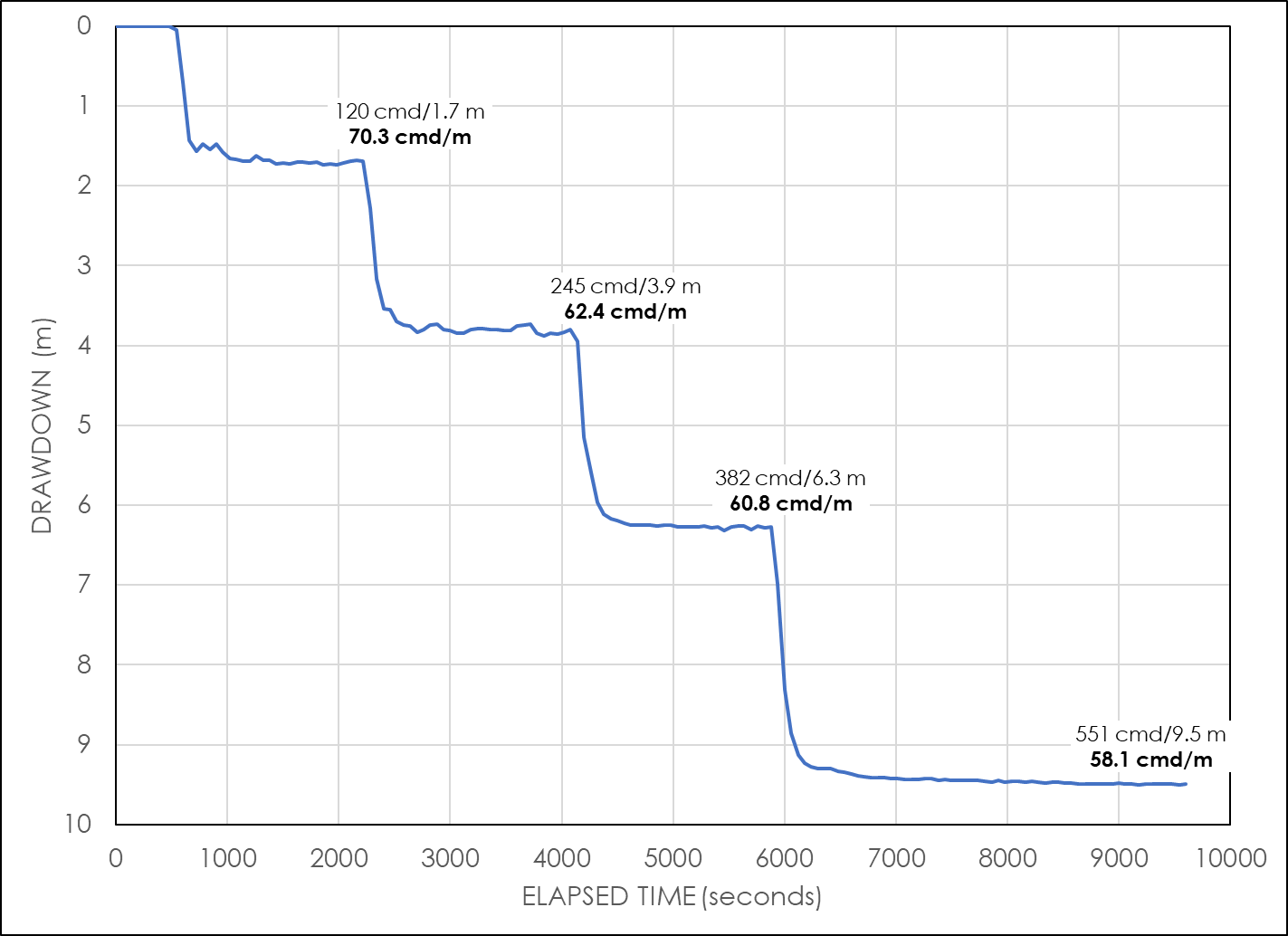
Figure 51 ‑ Time‑drawdown data for a step‑rate test with four pumping rates performed on a well in an unconfined aquifer in unconsolidated clastic sedimentary material.
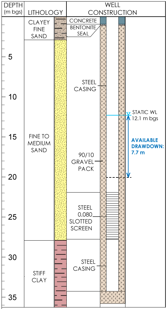
Figure 52 ‑ Lithology and well construction diagram showing the static water level and the available drawdown in the well, which in this case is defined as the water column above a point 1.5 m above the top of the screened interval.
Figure 51 shows time‑drawdown data for each step and indicates the stabilization of the water levels at each step. The specific capacity at each step is calculated based on the step pump rate and the final drawdown at each step; these are presented in Table 5 and on Figure 51. The specific capacity values range from 70.3 cmd/m at the lowest pumping rate (120 cmd) to 58.1 cmd/n at the highest pumping rate (551 cmd), which is consistent with the expectation of lower efficiency at higher pumping rates. The specific capacity at the highest pumping rate (58.1 cmd/m) is about 80 percent of the specific capacity at the lowest pumping rate (70.3 cmd/m), which indicates that the well construction is reasonably good but there is some inefficiency at desirable pumping rates.
The Remaining Available Drawdown column of Table 5 is the difference between the water level at the various pumping rates and the 19.8 m bgs drawdown limit established for the well. The table indicates that pumping at 551 cmd exceeds the drawdown limit; therefore, the optimal pumping rate is somewhere between 400 cmd and 551 cmd. The optimal pumping rate, or well yield, can therefore be determined by graphing the pumping rates versus the drawdowns at each step, establishing a best fit trendline to the data, and calculating the pumping rate (in this case, 452 cmd) for a drawdown that equals the available drawdown with no pumping (7.7 m) and results in zero remaining drawdown (Figure 53).
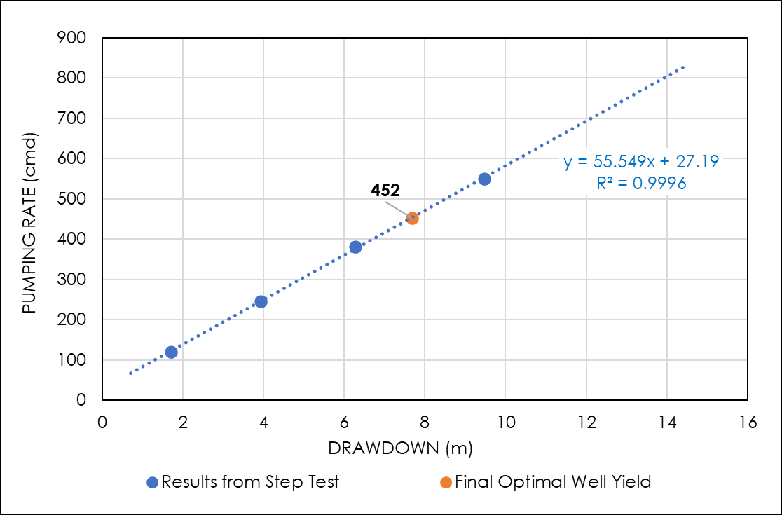
Figure 53 ‑ Graph of test pumping rate versus drawdown. The final optimal well yield is determined by interpolation to find the pumping rate for a drawdown of 7.7 m.
More details about step‑test procedures and data analysis can be found in An Introduction to Hydraulic Testing in Hydrogeology: Basic Pumping, Slug, and Packer Methods↗ by Woessner and others (2020), which is available as a free download from The Groundwater Project.