16.6 Modeling Fluid Flow in Fractures

A purely fractured system can be modeled using the cubic law and the assumptions that 1) all fluid flow is in the fractures, and 2) the fractures can be represented as a series of parallel plates—in other words, the fractures are all smooth‑walled and have constant apertures. The spacing and density of fractures in a volume of rock can be used to integrate the cubic law over the whole volume, so that a hydraulic conductivity tensor for the whole volume is calculated. There are also ways to factor in roughness and variations in aperture; usually these involve multiplying the cubic law by some factor that reduces the flow accordingly.

This method has some limitations. It has an implicit assumption that the fractures follow a constant spacing, or some spacing that varies in a predictable way. Also, it ignores flow in the matrix, which may or may not be a good assumption.

If the exact locations, extents, orientations, and hydraulic properties of all the fractures in a system are known with some degree of confidence, the system can be simulated using a model that contains and calculates flow in each fracture. This is used frequently in the petroleum industry for reservoirs that have been extensively studied through drilling and geophysics such that locations of the major fractures are known with some certainty. The obvious limitation with this is that, to get a meaningful model, you need to have lots of data and high confidence in those data. For many groundwater problems, this is not within the budget, thus those data are not available.

Stochastic means random or statistical. In stochastic models, the probability of occurrence of a fracture is input to the model rather than actual orientations. The model generates many possible fracture configurations and calculates flow for all of them to provide a range of flow results. These can be used where data is sparse and are most effective when it can be shown that the fractures follow some sort of predictable distribution.

Some numerical models incorporate a parallel‑plate or discrete fracture approach with a standard porous media model approach to simulate flow in a double‑porosity system. A difficult part of these models is characterizing the relationship between the fractures and the matrix blocks—a mathematical function must be specified that controls the flow of water from fractures to the matrix and vice‑versa. This function is most likely non‑linear and represents a process that is not well understood.

A simple way of modeling double‑porosity systems is by ignoring the fractures and developing equivalent hydraulic parameters that characterize the aquifer as a single porous medium. The idea is that, even though the system is fractured, the model contains a representative elemental volume (REV) of the formation or aquifer. This approach is used frequently, most likely because modelers don’t have enough data to meaningfully apply an alternative approach. This method works if the fractures are so numerous and well‑connected that the whole aquifer acts as an equivalent porous medium, but it does not work well if a few large fractures are controlling the flow system. Sometimes a few of the large fractures will be represented by extremely high permeability porous zones.

A more appropriate way of using the equivalent porous media approach is by establishing fracture domains, or areas in which the fractures have common characteristics—orientation, connectivity, and so on (Figure 134). Investigations (air photo, outcrop) can be used to establish regions with similar fracture characteristics. The parallel plate approach can be used to establish a hydraulic conductivity tensor for each region. These can then be input into a heterogeneous porous media model with variable anisotropy.

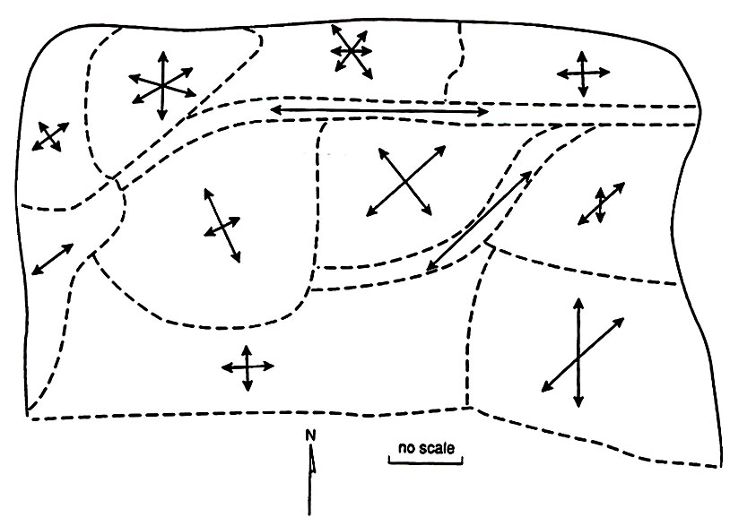
Figure 134 ‑ Hypothetical fracture domains in map view with arrows representing hypothetical fracture set directions within the delineated zones (reproduced courtesy of John M. Sharp, University of Texas, Austin).